Week 5: Model selection
PLS 206 — the code behind the lectures
One page for the whole week. It follows the slides (Week5_Model_Selection.pptx) in order, and has the code behind every figure and number in the lecture, with the output underneath.
To run it yourself, download either version and open it in RStudio. It reads the data straight from the course website, so there is no file to download and no working directory to set:
- Week5_Model_Selection.R: the plain script. Each block is tagged
[CORE],[HANDY], or[DEMO]in a comment. - Week5_Model_Selection.qmd: this page as a Quarto notebook (open in RStudio, run chunk by chunk, or click Render).
Every block of code on this page carries one of three labels:
- Core The analysis. Code you would run on your own data: fit the model, read the output, check the diagnostics, report it. Start here for the problem sets.
- Handy Useful, not essential. Wrangling, plotting, and small helpers that make the core easier. Worth knowing; skip on a first read.
- Demo For the lecture only. Simulated data, sums done by hand, and the code behind slide figures. It shows why the core works. Folded: click to open.
# install.packages(c("ggplot2", "MuMIn", "car", "MASS"))
library(ggplot2)
library(MuMIn)   # AICc(), model.sel(), dredge(), sw(), model.avg()
library(car)     # vif()
library(MASS)    # stepAIC()
Which tool for which question
| You want… | Use |
|---|---|
| A score for one model | AIC(m), AICc(m) (MuMIn), BIC(m) |
| To compare a few models you wrote down before looking | model.sel(m1, m2, m3) |
| A test for one nested pair | anova(m_small, m_big) |
| To find collinear predictors | vif(m) (car): drop the worst, refit, repeat |
| To search every subset (exploration) | options(na.action = "na.fail"), then dredge(full, fixed = ~ control) |
| How much support each variable has | sw(dd) |
| Estimates across the well-supported models | model.avg(get.models(dd, subset = delta < 2)) |
| To judge predictions | fit on part of the data, predict the rest |
Part A. Too many models
1) The data: the cover-crop farms
The cover-crop data from the Week 2 live coding: spring biomass (biomass, kg/ha) of the same cover crop on 50 farms, with each farm’s location, winter weather and soil. clay goes, because sand + silt + clay = 100 (Week 2). Simulated: only growing degree days (gdd) drives biomass, so we can check what each method finds.
farms <- read.csv("https://greymonroe.github.io/PLS_206/data/cover_crop.csv")
farms <- subset(farms, select = -c(farm, clay))
head(farms)
biomass latitude longitude elevation gdd tmean_winter tmin_coldest
1 2797 39.72 -120.70 358 894 7.4 -0.7
2 3582 41.62 -121.65 383 733 6.1 -2.8
3 2279 38.18 -119.94 695 728 7.3 -0.8
4 4789 38.14 -122.07 234 1047 11.2 3.3
5 5067 37.93 -120.53 286 1028 8.6 0.4
6 6026 37.27 -121.36 205 1262 10.8 3.0
frost_days rain_total rain_wettest rain_driest dry_spell sand silt soil_ph
1 34 396 83 15 45 54 28 7.7
2 43 662 150 32 25 21 17 7.0
3 40 562 149 24 34 43 38 7.3
4 21 597 112 23 27 35 32 6.5
5 22 820 207 39 24 25 37 7.7
6 22 784 183 31 19 43 18 7.1
organic_matter
1 1.6
2 1.9
3 2.5
4 2.4
5 2.5
6 2.1nrow(farms)[1] 50P <- setdiff(names(farms), "biomass") # the 15 candidate predictors
long <- do.call(rbind, lapply(P, function(v) data.frame(var = v, x = farms[[v]], biomass = farms$biomass)))
long$var <- factor(long$var, levels = P)
ggplot(long, aes(x, biomass / 1000)) +
geom_point(colour = "grey50", size = 1) +
facet_wrap(~ var, scales = "free_x", nrow = 3) +
labs(x = NULL, y = "Biomass (t/ha)") +
theme_classic()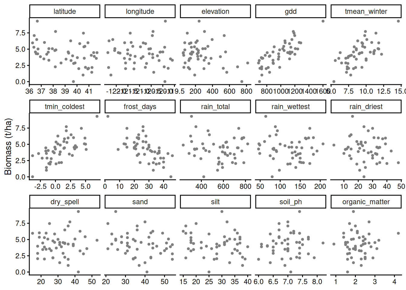
2) How many models could we fit?
Each predictor is in or out, so 15 predictors give 2^15 models, before any interactions or curves.
ncol(farms) - 1 # candidate predictors[1] 152^15 # possible models (each one in or out)[1] 327683) Add predictors: R² only goes up
Fit on 25 farms, add predictors one at a time, best first (the strongest correlation with biomass on those 25 farms), until all 15 are in. Keep the R² on the 25 farms and the prediction error (RMSE) on both halves.
Demo: fit on 25 farms, add predictors best first
set.seed(5)
tr <- sample(50, 25)                                          # the 25 farms we fit to
ord <- names(sort(-abs(cor(farms[tr, ])[P, "biomass"])))      # predictors, best first
rmse <- function(obs, pred) sqrt(mean((obs - pred)^2))
of <- do.call(rbind, lapply(0:15, function(k) {
  fm <- if (k == 0) biomass ~ 1 else reformulate(ord[1:k], "biomass")
  m <- lm(fm, data = farms[tr, ])
  data.frame(k = k, r2 = summary(m)$r.squared,
             train = rmse(farms$biomass[tr], fitted(m)),
             test  = rmse(farms$biomass[-tr], predict(m, farms[-tr, ])))
}))
round(of, 3)    # R-squared 0.57 with 1 predictor, 0.88 with 15
k r2 train test
1 0 0.000 1584.268 1950.863
2 1 0.571 1037.808 1163.579
3 2 0.703 862.676 1397.993
4 3 0.733 818.588 1629.398
5 4 0.733 818.402 1621.646
6 5 0.766 766.264 1689.005
7 6 0.770 759.885 1669.620
8 7 0.770 759.847 1672.966
9 8 0.782 739.895 1787.303
10 9 0.799 710.736 1920.947
11 10 0.799 710.385 1916.919
12 11 0.811 689.327 1942.501
13 12 0.818 675.596 1909.517
14 13 0.828 656.552 2148.164
15 14 0.835 642.956 2290.458
16 15 0.877 555.474 2572.571Demo: fit on 25 farms, add predictors best first
ggplot(of, aes(k, r2)) +
  geom_line(colour = "blue", linewidth = 1) + geom_point(colour = "blue", size = 2) +
  scale_y_continuous(limits = c(0, 1)) +
  labs(x = "Number of predictors in the model", y = "R² on the 25 farms it was fitted to") +
  theme_classic()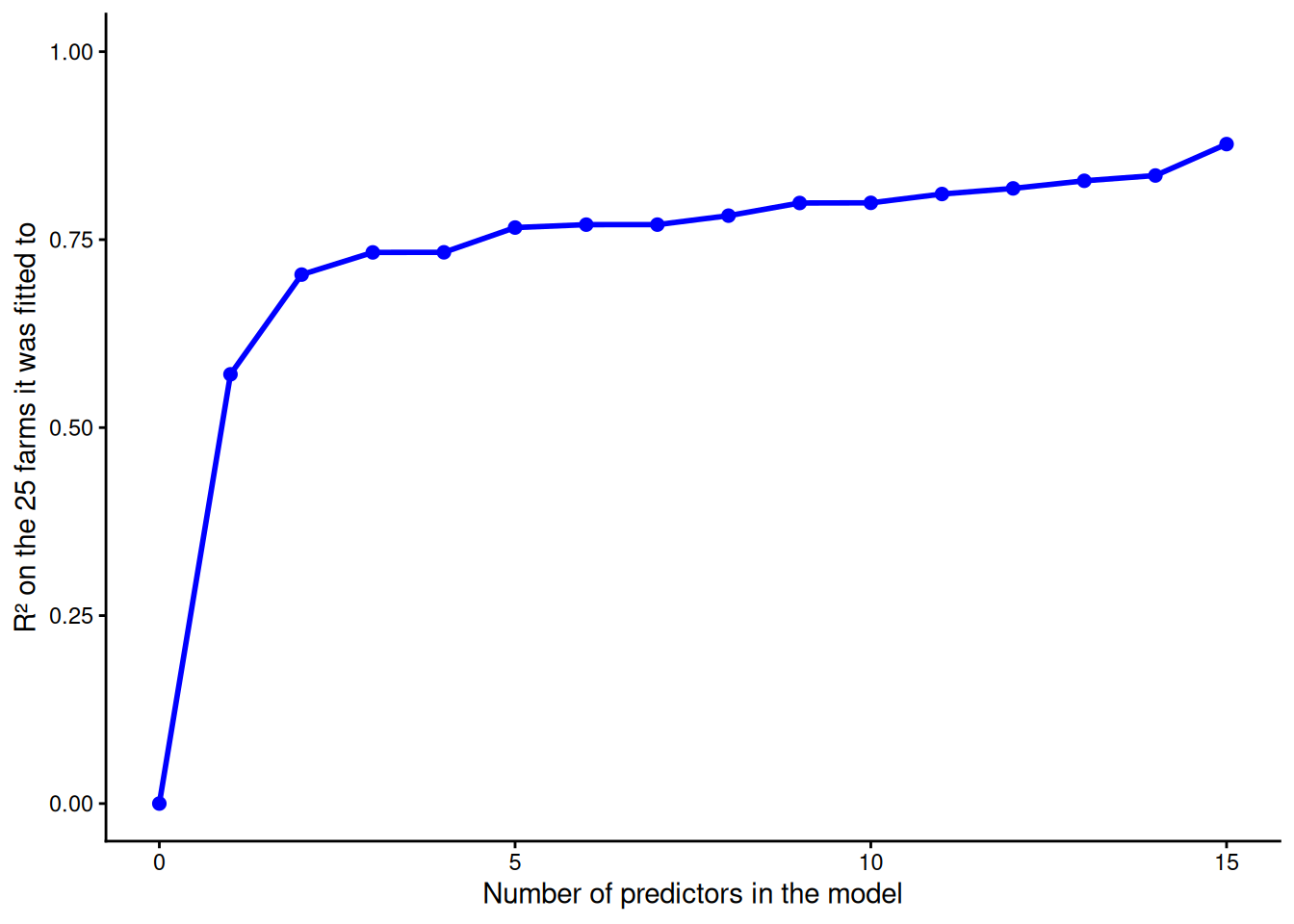
4) …but the other 25 farms get worse
The error on the 25 farms the model was fitted to falls from 1.04 to 0.56 t/ha. On the other 25 farms it is lowest with one predictor (gdd, 1.16 t/ha) and reaches 2.57 t/ha with all 15.
Demo: prediction error on both halves, and predicted vs observed
ol <- rbind(data.frame(k = of$k, err = of$train, set = "the 25 farms it was fitted to"),
            data.frame(k = of$k, err = of$test,  set = "the other 25 farms"))
ggplot(ol, aes(k, err / 1000, colour = set)) +
  geom_line(linewidth = 1) + geom_point(size = 2) +
  scale_colour_manual(values = c("blue", "red"), name = "Prediction error on") +
  expand_limits(y = 0) +
  labs(x = "Number of predictors in the model", y = "Prediction error, RMSE (t/ha)") +
  theme_classic()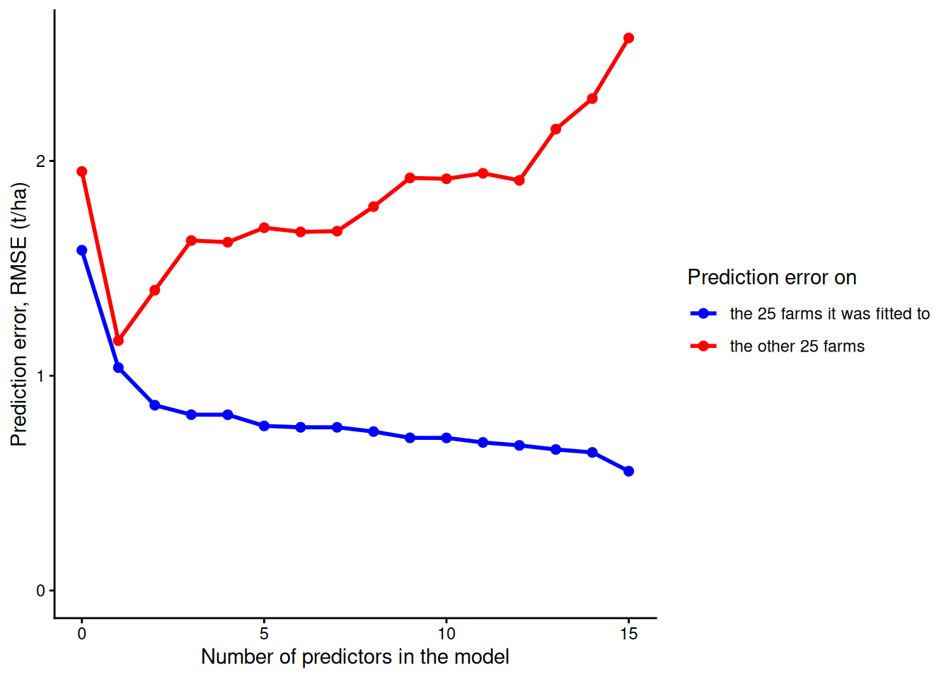
Demo: prediction error on both halves, and predicted vs observed
of$k[which.min(of$test)] # best on new farms: 1 predictor[1] 1Demo: prediction error on both halves, and predicted vs observed
# predicted vs observed on the other 25 farms, 1 vs 15 predictors
pv <- do.call(rbind, lapply(c(1, 15), function(k) {
  m <- lm(reformulate(ord[1:k], "biomass"), data = farms[tr, ])
  data.frame(model = paste(k, "predictor(s)"), obs = farms$biomass[-tr], pred = predict(m, farms[-tr, ]))
}))
ggplot(pv, aes(obs / 1000, pred / 1000)) +
  geom_abline(linetype = 2, colour = "grey50") +
  geom_point(colour = "red") +
  facet_wrap(~ model) + coord_equal() +
  labs(x = "Observed biomass, the other 25 farms (t/ha)", y = "Predicted (t/ha)") +
  theme_classic()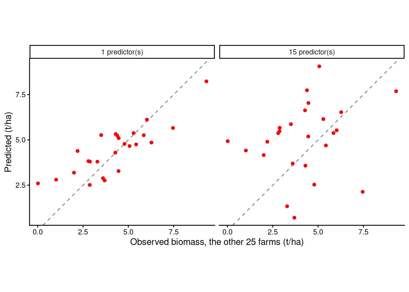
Overfitting: the extra coefficients describe the noise in the first 25 farms, and that noise is not in the next 25.
5) What is the model for?
Three goals, each with its own way to choose (Tredennick et al. 2021, Ecology):
| Goal | How to choose | Where |
|---|---|---|
| Explore: many variables, no strong expectations | search all subsets; the findings are new hypotheses | Part D |
| Test ideas: you had them before the data | a few models written first; AIC weights | Part C |
| Predict: new places, years, plants | held-out data, cross-validation | Part F, Week 6 |
All three need a score that does not reward complexity for free. That is AIC (Part B).
Part B. Scoring models
6) Likelihood, one farm at a time
Plot the raw data first, then the model on top.
# fitted values with a 95% CI, for any lm() or glm(), on the scale of y
fit_ci <- function(model, newdata, level = 0.95) {
  p <- predict(model, newdata = newdata, se.fit = TRUE)   # link scale for a glm
  q <- if (inherits(model, "glm")) qnorm(1 - (1 - level) / 2) else qt(1 - (1 - level) / 2, df.residual(model))
  inv <- family(model)$linkinv                            # identity for lm()
  fit <- as.numeric(p$fit); se <- as.numeric(p$se.fit)
  data.frame(newdata, fit = inv(fit), lwr = inv(fit - q * se), upr = inv(fit + q * se))
}
g_gdd <- data.frame(gdd = seq(min(farms$gdd), max(farms$gdd), length.out = 100))

p_gdd <- ggplot(farms, aes(gdd, biomass / 1000)) +
  geom_point(colour = "grey50") +
  labs(x = "Growing degree days (Oct to Mar)", y = "Biomass (t/ha)") +
  theme_classic()
p_gdd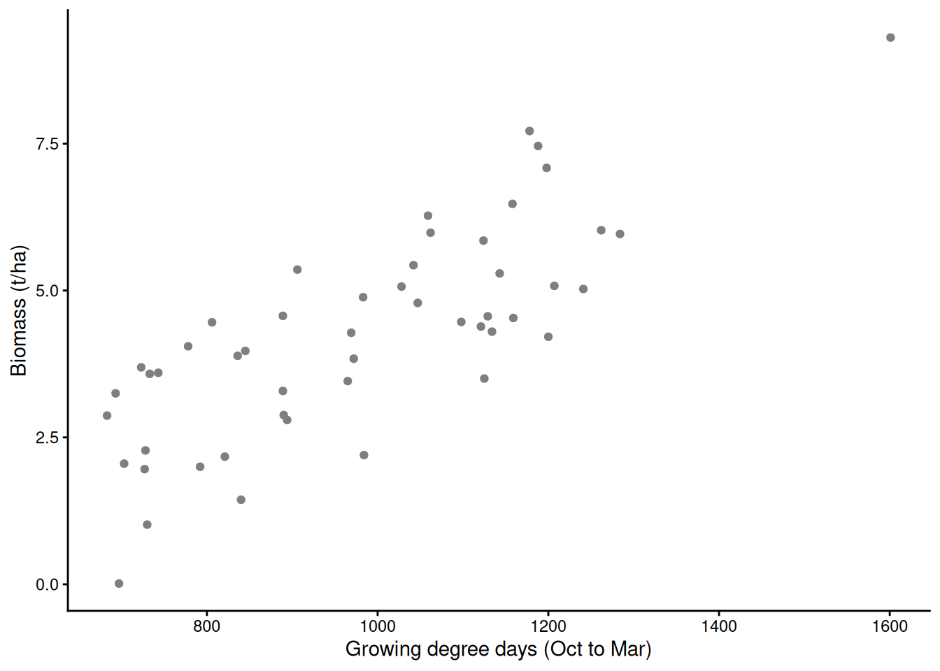
m_temp <- lm(biomass ~ gdd, data = farms)
logLik(m_temp)     # -420.47, df = 3: intercept, slope, and sigma
'log Lik.' -420.4669 (df=3)ci_temp <- fit_ci(m_temp, g_gdd)
p_gdd +
geom_ribbon(data = ci_temp, aes(gdd, ymin = lwr / 1000, ymax = upr / 1000), inherit.aes = FALSE, fill = "blue", alpha = 0.2) +
geom_line(data = ci_temp, aes(gdd, fit / 1000), colour = "blue", linewidth = 1)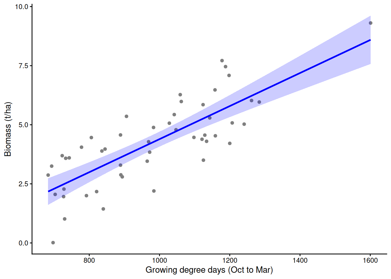
The model puts a normal bell around the line at each farm’s degree days, with width sigma. A farm’s likelihood is the height of its bell where the farm actually landed: high if the model expected it, low if not. The likelihood of the data is the product of the 50 heights; we add their logs instead. It is the probability of the data under the model, not the probability that the model is true. logLik() uses the maximum-likelihood sigma, which divides by n, not n − 2.
sigma <- sqrt(mean(resid(m_temp)^2))                  # width of the bell

# one farm: the height of the normal curve at its biomass
y <- farms$biomass[4]; y_hat <- fitted(m_temp)[[4]]
1 / (sigma * sqrt(2 * pi)) * exp(-(y - y_hat)^2 / (2 * sigma^2))
[1] 0.0003665691dnorm(y, mean = y_hat, sd = sigma) # the same, built in[1] 0.0003665691# every farm at once
scores <- dnorm(farms$biomass, mean = fitted(m_temp),
sd = sigma, log = TRUE) # log height, each farm
round(range(scores), 2) # worst and best farm[1] -10.07 -7.91sum(scores) # = logLik(m_temp)[1] -420.4669A worse model expects the data less. The null model gives every farm the same prediction, so its bell is wide and low:
m_null <- lm(biomass ~ 1, data = farms)
logLik(m_null)     # -445.07, lower than -420.47
'log Lik.' -445.0677 (df=2)lm() and glm() choose the coefficients that make the observed data most probable: maximum likelihood. Try every slope, and log L peaks at the slope lm() reports:
Demo: log L for every slope (the peak is the lm() slope)
slopes <- seq(0, 14, by = 0.05)
ll <- sapply(slopes, function(b) {
  a <- mean(farms$biomass) - b * mean(farms$gdd)      # best intercept for this slope
  r <- farms$biomass - a - b * farms$gdd
  sum(dnorm(r, 0, sqrt(mean(r^2)), log = TRUE))
})
slopes[which.max(ll)]     # 7.00, the lm() slope (6.99) to the grid step
[1] 7Demo: log L for every slope (the peak is the lm() slope)
plot(slopes, ll, type = "l", xlab = "Slope tried", ylab = "log L")
abline(v = coef(m_temp)["gdd"], col = "blue", lty = 2)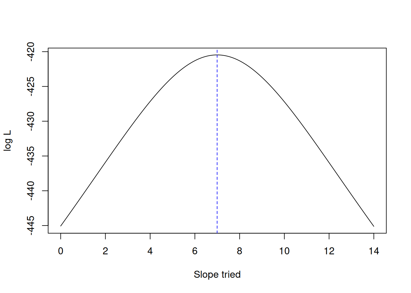
For yes/no data there are no bells: each record’s likelihood is the probability the model gave to what actually happened, p if it happened and 1 − p if not.
Demo: likelihood of a logistic regression by hand (Wednesday’s pistachios)
pis_l <- read.csv("https://greymonroe.github.io/PLS_206/data/pistacia_niche.csv")
pis_l$y <- as.integer(pis_l$species_short == "terebinthus")
m_bin <- glm(y ~ bio1_annual_mean_temp, family = binomial, data = pis_l)
p_ter <- fitted(m_bin)                                # P(terebinthus) for each record
sum(log(ifelse(pis_l$y == 1, p_ter, 1 - p_ter)))              # = logLik(m_bin)
[1] -4047.941Demo: likelihood of a logistic regression by hand (Wednesday’s pistachios)
logLik(m_bin)'log Lik.' -4047.941 (df=2)Demo: the bells on the slides
sig <- sigma
xs <- c(750, 1000, 1250)
dens <- do.call(rbind, lapply(xs, function(x0) {
  mu <- predict(m_temp, data.frame(gdd = x0))
  y <- seq(mu - 3 * sig, mu + 3 * sig, length.out = 200)
  data.frame(x0 = x0, y = y, x = x0 + 9e4 * dnorm(y, mu, sig))
}))
ggplot(farms, aes(gdd, biomass / 1000)) +
  geom_point(colour = "grey50") +
  geom_abline(intercept = coef(m_temp)[1] / 1000, slope = coef(m_temp)[2] / 1000, colour = "blue", linewidth = 1) +
  geom_path(data = dens, aes(x, y / 1000, group = x0), colour = "orange", linewidth = 1) +
  geom_vline(xintercept = xs, colour = "orange", linetype = 3) +
  labs(x = "Growing degree days (Oct to Mar)", y = "Biomass (t/ha)") +
  theme_classic()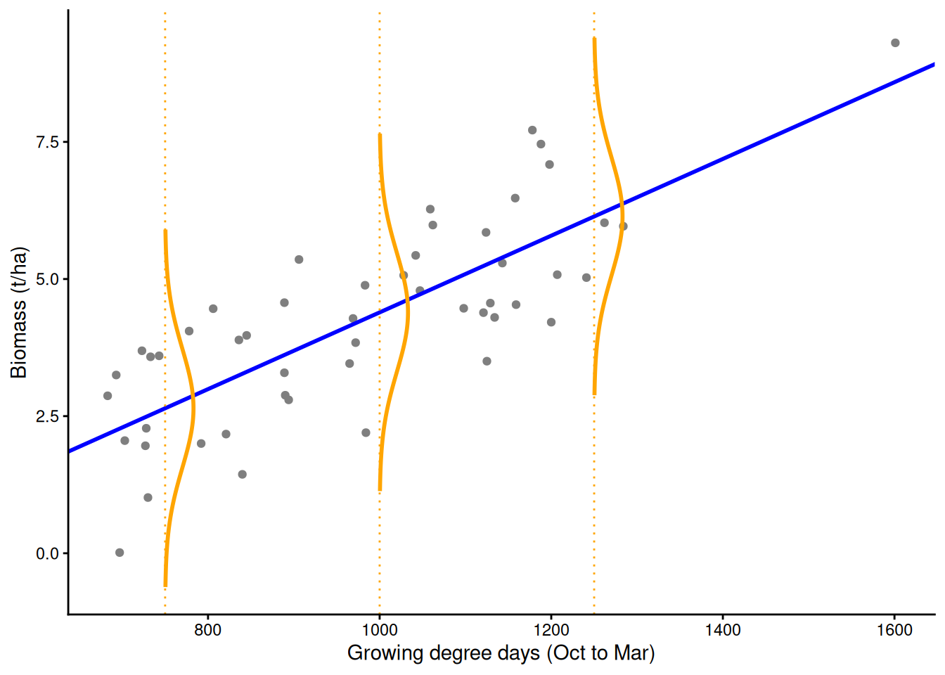
7) AIC = misfit + a price for each parameter
AIC = −2 log L + 2k. Here 840.93 + 2 × 3 = 846.93. AIC() gives the same, as long as k counts sigma.
AIC(m_temp)[1] 846.9337-2 * as.numeric(logLik(m_temp)) + 2 * 3 # k = 3: intercept, slope, sigma[1] 846.9337attr(logLik(m_temp), "df") # the k that R uses[1] 38) The null model
No predictors: k = 2 (the mean and sigma). AIC = −2 × −445.07 + 4 = 894.1, about 47 worse than the gdd model.
m_null <- lm(biomass ~ 1, data = farms)
logLik(m_null)
'log Lik.' -445.0677 (df=2)AIC(m_null)[1] 894.1354AIC(m_null) - AIC(m_temp)[1] 47.20163ci_null <- fit_ci(m_null, g_gdd)
p_gdd +
geom_ribbon(data = ci_null, aes(gdd, ymin = lwr / 1000, ymax = upr / 1000), inherit.aes = FALSE, fill = "grey40", alpha = 0.2) +
geom_line(data = ci_null, aes(gdd, fit / 1000), colour = "grey30", linewidth = 1) +
geom_line(data = ci_temp, aes(gdd, fit / 1000), colour = "blue", linewidth = 1)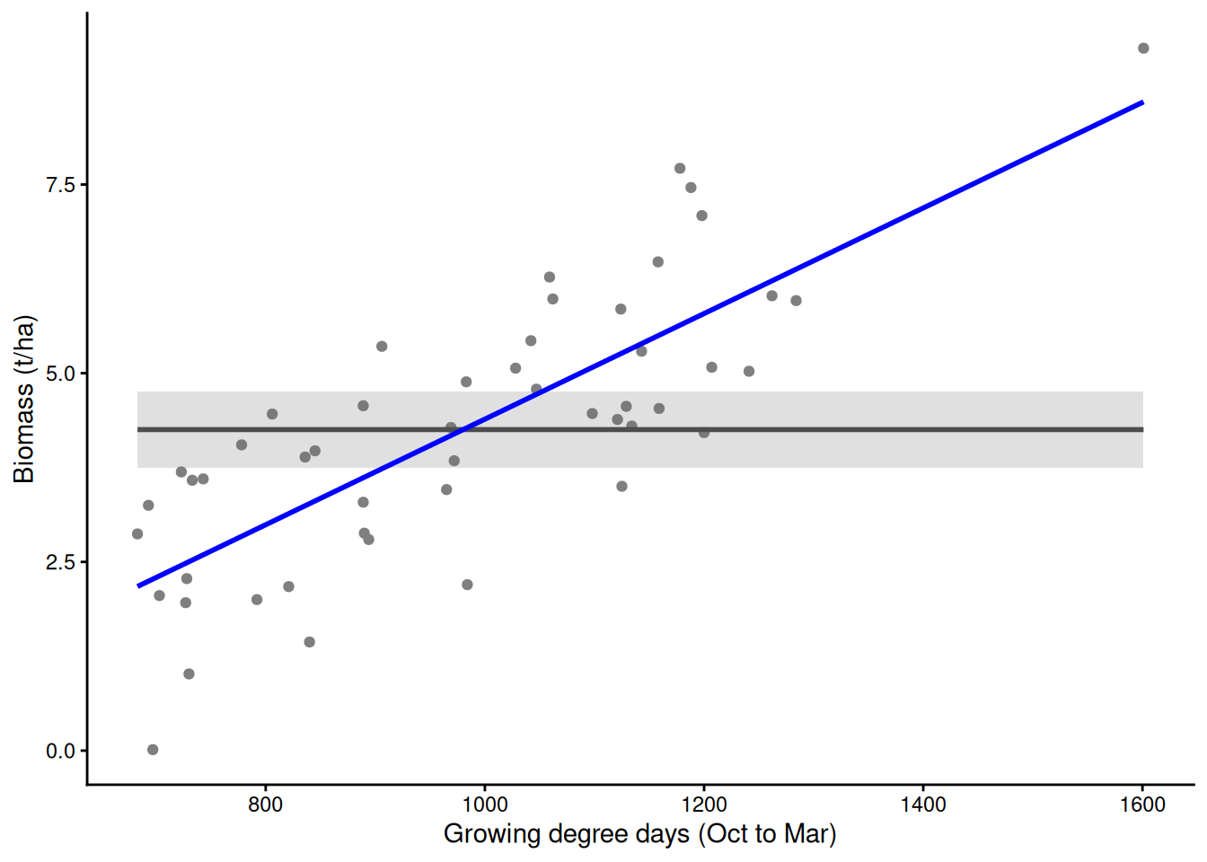
9) Misfit falls, the penalty rises, AIC finds the balance
All 50 farms, adding predictors best first. The misfit drops sharply when gdd comes in, then barely moves; the penalty rises by 2 with every predictor. AIC is lowest at 2 predictors.
Demo: misfit, penalty and AIC as predictors are added
ord50 <- names(sort(-abs(cor(farms)[P, "biomass"])))     # best first, all 50 farms
fp <- do.call(rbind, lapply(0:15, function(k) {
  m <- lm(if (k == 0) biomass ~ 1 else reformulate(ord50[1:k], "biomass"), data = farms)
  h <- hatvalues(m)
  data.frame(k = k, misfit = -2 * as.numeric(logLik(m)), penalty = 2 * attr(logLik(m), "df"),
             aic = AIC(m), bic = BIC(m),
             loo = sqrt(mean((resid(m) / (1 - h))^2)))   # leave-one-out error, used in Part F
}))
fp$k[which.min(fp$aic)]    # 2 predictors
[1] 2Demo: misfit, penalty and AIC as predictors are added
fl <- rbind(data.frame(k = fp$k, v = fp$misfit - min(fp$misfit), part = "misfit: -2 log L"),
            data.frame(k = fp$k, v = fp$penalty - min(fp$penalty), part = "penalty: 2k"),
            data.frame(k = fp$k, v = fp$aic - min(fp$aic), part = "AIC = misfit + penalty"))
fl$part <- factor(fl$part, levels = unique(fl$part))
ggplot(fl, aes(k, v, colour = part)) +
  geom_line(linewidth = 1) + geom_point(size = 2) +
  scale_colour_manual(values = c("blue", "red", "black"), name = NULL) +
  labs(x = "Number of predictors in the model", y = "Change from its lowest value") +
  theme_classic()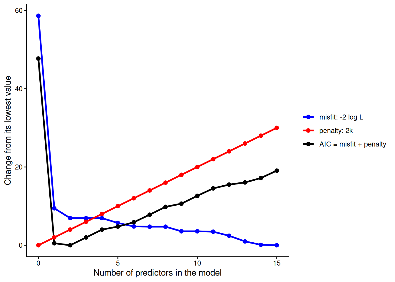
10) ΔAIC and Akaike weights
Only differences mean anything: ΔAIC = AIC − the lowest AIC in the set. Rules of thumb (Burnham and Anderson): within about 2, about equally supported; 4 to 7, clearly less; over 10, essentially none. Each model’s weight is exp(−Δ/2), divided by the total, so the weights add to 1. Here are three of the models from Part C (m_tm adds rain, m_all adds rain and soil):
Demo: delta and weights by hand
m_tm  <- lm(biomass ~ gdd + rain_total, data = farms)
m_all <- lm(biomass ~ gdd + rain_total + organic_matter + soil_ph, data = farms)
a <- c(m_temp = AICc(m_temp), m_tm = AICc(m_tm), m_all = AICc(m_all))
delta <- a - min(a)
w <- exp(-delta / 2) / sum(exp(-delta / 2))
round(cbind(AICc = a, delta, weight = w), 2)    # deltas 0, 2.11, 5.89; weights 0.71, 0.25, 0.04
AICc delta weight
m_temp 847.46 0.00 0.71
m_tm 849.56 2.11 0.25
m_all 853.35 5.89 0.0411) AICc: a correction for small samples
AICc = AIC + 2k(k + 1) / (n − k − 1). Large when k is close to n, fading as n grows. Use it when n/k is below about 40; with 50 farms it adds about half a point.
AICc(m_temp) # MuMIn[1] 847.4555Demo: AICc by hand
n <- nobs(m_temp); k <- 3
AIC(m_temp) + 2 * k * (k + 1) / (n - k - 1)
[1] 847.455512) BIC: a stiffer price
BIC = −2 log L + k log(n). With 50 farms, log(50) = 3.91 per parameter instead of 2; with the 6,299 Pistacia records in Part D, 8.7. BIC picks smaller models than AIC, and the difference grows with n. AIC aims at the model that predicts new data best; BIC at the true model, if it is in the set.
BIC(m_temp)[1] 852.6698-2 * as.numeric(logLik(m_temp)) + 3 * log(50)[1] 852.6698log(c(50, 6299)) # BIC's price per parameter; AIC's is 2[1] 3.912023 8.748146Demo: the penalty per parameter as n grows
pen <- data.frame(n = exp(seq(log(5), log(20000), length.out = 300)))
ggplot(pen, aes(n, log(n))) +
  geom_line(colour = "purple", linewidth = 1) +
  geom_hline(yintercept = 2, colour = "blue", linewidth = 1) +
  annotate("point", x = c(50, 6299), y = log(c(50, 6299)), size = 3) +
  annotate("text", x = 3000, y = 1.5, label = "AIC: 2 per parameter", colour = "blue") +
  annotate("text", x = 200, y = 7.5, label = "BIC: log(n) per parameter", colour = "purple") +
  scale_x_log10() +
  labs(x = "Sample size, n (log scale)", y = "Penalty per parameter") +
  theme_classic()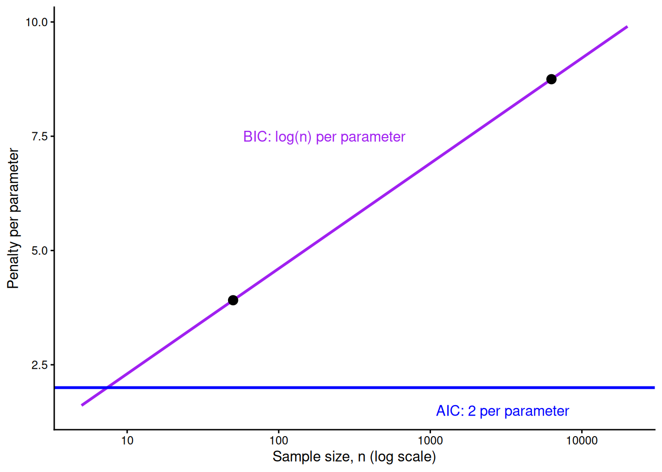
Part C. Testing ideas
13) Ideas first, then models: model.sel()
Three ideas about what limits cover-crop growth over winter, each written as a model before looking: temperature (gdd), moisture (rain_total), soil (organic_matter + soil_ph). Add the combinations that make sense and the null. model.sel() fits nothing itself: it ranks the models you give it by AICc, with delta and weights.
m_null  <- lm(biomass ~ 1, data = farms)
m_temp  <- lm(biomass ~ gdd, data = farms)
m_moist <- lm(biomass ~ rain_total, data = farms)
m_soil  <- lm(biomass ~ organic_matter + soil_ph, data = farms)
m_tm    <- lm(biomass ~ gdd + rain_total, data = farms)
m_all   <- lm(biomass ~ gdd + rain_total + organic_matter + soil_ph, data = farms)
ms <- model.sel(m_null, m_temp, m_moist, m_soil, m_tm, m_all)
round(as.data.frame(ms)[, c("df", "logLik", "AICc", "delta", "weight")], 2)
df logLik AICc delta weight
m_temp 3 -420.47 847.46 0.00 0.71
m_tm 4 -420.34 849.56 2.11 0.25
m_all 6 -419.70 853.35 5.89 0.04
m_null 2 -445.07 894.39 46.94 0.00
m_moist 3 -444.68 895.88 48.43 0.00
m_soil 4 -444.83 898.55 51.10 0.00Temperature alone is best (weight 0.71). Temperature + moisture is 2.11 behind with almost the same log likelihood: the gap is the penalty for one more parameter. Moisture alone and soil alone are worse than the null.
ms # the full table: coefficients of every modelModel selection table
(Int) gdd ran_ttl org_mtt sol_ph df logLik AICc delta weight
m_temp -2603 6.994 3 -420.467 847.5 0.00 0.714
m_tm -2289 6.955 -0.4959 4 -420.337 849.6 2.11 0.249
m_all -991 7.097 -0.3956 200.2 -274.8 6 -419.698 853.3 5.89 0.037
m_null 4253 2 -445.068 894.4 46.94 0.000
m_moist 5024 -1.3900 3 -444.681 895.9 48.43 0.000
m_soil 1846 173.6 291.1 4 -444.831 898.6 51.10 0.000
Models ranked by AICc(x) model.sel(m_null, m_temp, m_moist, m_soil, m_tm, m_all, rank = BIC) # ranked by BIC insteadModel selection table
(Int) gdd ran_ttl org_mtt sol_ph df logLik BIC delta weight
m_temp -2603 6.994 3 -420.467 852.7 0.00 0.857
m_tm -2289 6.955 -0.4959 4 -420.337 856.3 3.65 0.138
m_all -991 7.097 -0.3956 200.2 -274.8 6 -419.698 862.9 10.20 0.005
m_null 4253 2 -445.068 898.0 45.29 0.000
m_moist 5024 -1.3900 3 -444.681 901.1 48.43 0.000
m_soil 1846 173.6 291.1 4 -444.831 905.3 52.64 0.000
Models ranked by BIC(x) 14) The evidence, as weights
wd <- data.frame(model = rownames(ms), weight = ms$weight)
wd$model <- factor(wd$model, levels = rev(wd$model))
ggplot(wd, aes(weight, model)) +
  geom_col(fill = "blue", width = 0.6) +
  geom_text(aes(label = sprintf("%.2f", weight)), hjust = -0.2) +
  scale_x_continuous(limits = c(0, 1)) +
  labs(x = "Akaike weight", y = NULL) +
  theme_classic()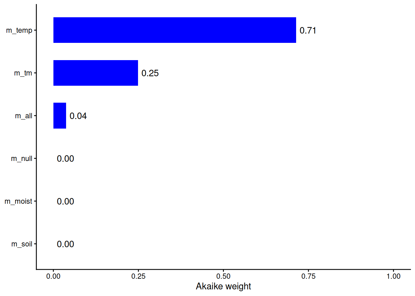
15) Nested models: anova() and AIC agree
m_tm is m_temp plus one term, so the F test from Week 2 works too: p = 0.62 and ΔAICc = 2.11, the same conclusion.
anova(m_temp, m_tm) # does adding moisture help?Analysis of Variance Table
Model 1: biomass ~ gdd
Model 2: biomass ~ gdd + rain_total
Res.Df RSS Df Sum of Sq F Pr(>F)
1 48 58986591
2 47 58681162 1 305428 0.2446 0.623216) Not nested? Only AIC can compare them
Moisture vs soil: neither model is the other plus extra terms. anova() runs, but gives a negative sum of squares and no test. AIC can compare any models fitted to the same rows with the same response.
anova(m_moist, m_soil) # moisture vs soil: not nestedAnalysis of Variance Table
Model 1: biomass ~ rain_total
Model 2: biomass ~ organic_matter + soil_ph
Res.Df RSS Df Sum of Sq F Pr(>F)
1 48 155377480
2 47 156318053 1 -940573 AICc(m_moist) - AICc(m_soil)[1] -2.66891117) Some terms stay, no matter what
Not up for selection: design terms (blocks, plots: the analysis must match how the data were collected), known controls (sampling effort in Part D, kept with fixed =), and the main effects under any interaction or the linear term under a quadratic (dredge() respects this by default).
18) Same response: log(y) and y cannot be compared
m_raw <- lm(biomass ~ gdd, data = farms)
m_log <- lm(log(biomass) ~ gdd, data = farms)
AIC(m_raw, m_log)        # 846.9 vs 123.1: different units, not a better model
df AIC
m_raw 3 846.9337
m_log 3 123.1217The likelihood of log biomass is in different units from the likelihood of biomass. Pick the scale first, from the residuals (Week 2), then compare models on that scale.
19) Same rows: missing values change n
Suppose three soil tests were lost. lm() quietly drops those farms from any model that uses soil_ph, so that model is scored on 47 farms and the other on 50.
farms_na <- farms
farms_na$soil_ph[c(3, 17, 29)] <- NA    # suppose 3 soil tests were lost
m_a <- lm(biomass ~ gdd, data = farms_na)
m_b <- lm(biomass ~ gdd + soil_ph, data = farms_na)
c(nobs(m_a), nobs(m_b))
[1] 50 47AIC(m_a, m_b) # m_b looks 48 better only because it has 3 fewer farms df AIC
m_a 3 846.9337
m_b 4 799.1344The fix: drop the incomplete rows once, before fitting any model.
farms_cc <- na.omit(farms_na)
m_a <- lm(biomass ~ gdd, data = farms_cc)
m_b <- lm(biomass ~ gdd + soil_ph, data = farms_cc)
c(nobs(m_a), nobs(m_b))
[1] 47 47AIC(m_a, m_b) df AIC
m_a 3 797.8171
m_b 4 799.134420) Report the table, not just the winner
Report the candidate set and the table (k, AICc, ΔAICc, weight), then the best model the usual way: coefficients with confidence intervals and a plot of the fit with the raw data (section 6).
round(as.data.frame(ms)[, c("df", "AICc", "delta", "weight")], 2) df AICc delta weight
m_temp 3 847.46 0.00 0.71
m_tm 4 849.56 2.11 0.25
m_all 6 853.35 5.89 0.04
m_null 2 894.39 46.94 0.00
m_moist 3 895.88 48.43 0.00
m_soil 4 898.55 51.10 0.00summary(m_temp)
Call:
lm(formula = biomass ~ gdd, data = farms)

Residuals:
    Min      1Q  Median      3Q     Max
-2259.5  -828.5  -149.7   972.0  2078.2

Coefficients:
             Estimate Std. Error t value Pr(>|t|)
(Intercept) -2602.600    780.417  -3.335  0.00165 **
gdd             6.994      0.780   8.967 7.93e-12 ***
---
Signif. codes:  0 '***' 0.001 '**' 0.01 '*' 0.05 '.' 0.1 ' ' 1

Residual standard error: 1109 on 48 degrees of freedom
Multiple R-squared:  0.6262,    Adjusted R-squared:  0.6184
F-statistic: 80.41 on 1 and 48 DF, p-value: 7.925e-12confint(m_temp) 2.5 % 97.5 %
(Intercept) -4171.733447 -1033.466302
gdd 5.426116 8.562702Part D. Exploring
21) The data: two Mediterranean pistachios
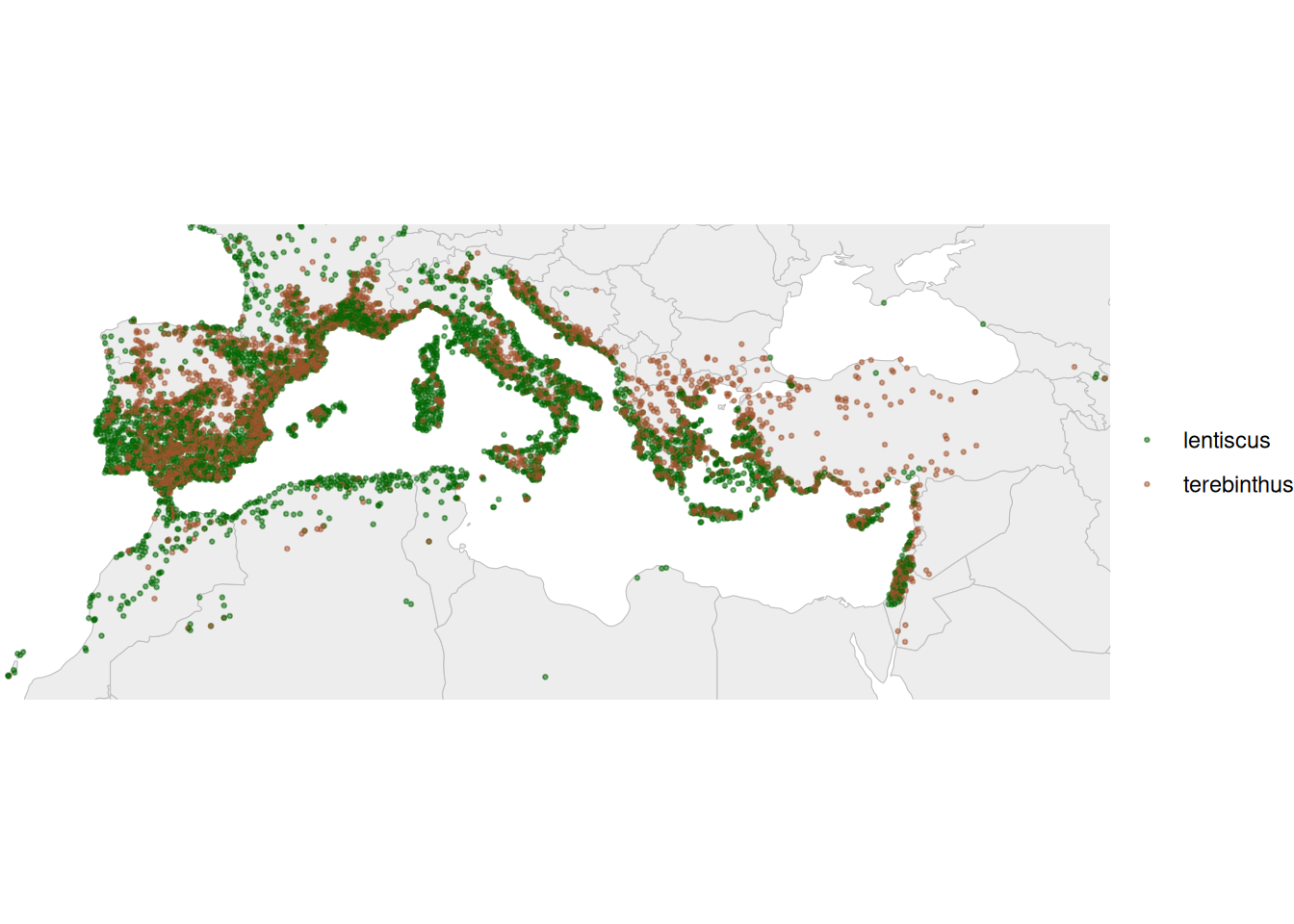
Pistacia lentiscus (mastic tree, evergreen) and P. terebinthus (turpentine tree, deciduous), wild relatives of the pistachio around the Mediterranean. 6,299 GBIF records with the 19 WorldClim bioclimatic variables at each spot. The response is y = 1 for terebinthus, 0 for lentiscus: a logistic regression (Week 3).
pis <- read.csv("https://greymonroe.github.io/PLS_206/data/pistacia_niche.csv")
names(pis) <- sub("^(bio[0-9]+)_.*", "\\1", names(pis))   # bio1 ... bio19
pis$y <- as.integer(pis$species_short == "terebinthus")
table(pis$species_short)
  lentiscus terebinthus
3678 2621 length(unique(pis$country))[1] 45Demo: the map (needs the maps package)
# install.packages("maps")
if (requireNamespace("maps", quietly = TRUE)) {
  world <- map_data("world")
  print(ggplot() +
    geom_polygon(data = world, aes(long, lat, group = group), fill = "grey93", colour = "grey75", linewidth = 0.2) +
    geom_point(data = pis, aes(lon, lat, colour = species_short), size = 0.5, alpha = 0.5) +
    scale_colour_manual(values = c(lentiscus = "darkgreen", terebinthus = "sienna"), name = NULL) +
    coord_quickmap(xlim = c(-12, 44), ylim = c(28, 47)) +
    theme_void())
}
22) 19 climate variables, all tangled
The species differ, but overlap a lot, and the 19 variables are built from the same monthly temperatures and rainfall.
bios <- paste0("bio", 1:19)
v4 <- c(bio1 = "Annual mean temp (°C)", bio6 = "Coldest-month min (°C)", bio4 = "Temp seasonality", bio12 = "Annual rain (mm)")
dl <- do.call(rbind, lapply(names(v4), function(v) data.frame(var = v4[[v]], x = pis[[v]], species = pis$species_short)))
dl$var <- factor(dl$var, levels = v4)
ggplot(dl, aes(x, fill = species, colour = species)) +
  geom_density(alpha = 0.3) +
  facet_wrap(~ var, scales = "free", nrow = 1) +
  scale_fill_manual(values = c("darkgreen", "sienna")) + scale_colour_manual(values = c("darkgreen", "sienna")) +
  labs(x = NULL) +
  theme_classic() + theme(legend.position = "bottom")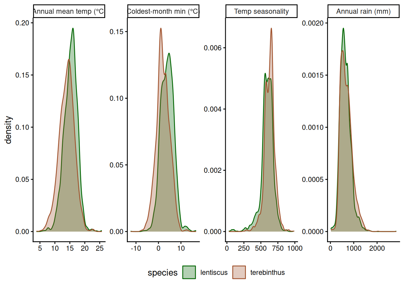
round(cor(pis[bios])[1:6, 1:6], 2) bio1 bio2 bio3 bio4 bio5 bio6
bio1 1.00 -0.02 0.21 -0.27 0.63 0.86
bio2 -0.02 1.00 0.66 0.36 0.65 -0.41
bio3 0.21 0.66 1.00 -0.43 0.28 0.11
bio4 -0.27 0.36 -0.43 1.00 0.39 -0.63
bio5 0.63 0.65 0.28 0.39 1.00 0.19
bio6 0.86 -0.41 0.11 -0.63 0.19 1.00A first model: species ~ temperature. Before choosing among 19 variables, one logistic regression (Week 3). Each record’s likelihood is the probability the model gave to what happened: the curve’s height for a terebinthus, 1 minus it for a lentiscus.
m_1 <- glm(y ~ bio1, family = binomial, data = pis)
p_ter <- fitted(m_1)                                   # P(terebinthus), each record
sum(log(ifelse(pis$y == 1, p_ter, 1 - p_ter)))         # likelihood by hand
[1] -4047.941logLik(m_1) # the same'log Lik.' -4047.941 (df=2)23) Throw everything in? bio7 is bio5 − bio6
All 19 in one logistic regression: three coefficients near ±30,000, for variables measured in degrees. bio7 (annual temperature range) is bio5 (warmest-month maximum) − bio6 (coldest-month minimum), so no data can separate the three.
m_all <- glm(y ~ ., family = binomial,
             data = pis[, c("y", paste0("bio", 1:19))])
round(coef(m_all)[c("bio5", "bio6", "bio7")])
bio5 bio6 bio7
-29776 29775 29776 range(pis$bio7 - (pis$bio5 - pis$bio6)) # bio7 IS bio5 - bio6[1] -1.907349e-06 1.907349e-06Before going on: the sampling-effort control (section 26) on a log scale, the records that have it, and the climate variables in SD units (scale()) so their coefficients compare. Keep the means and SDs to put the results back in raw units (section 32).
pis$effort <- log10(pis$plant_obs_effort)
pis <- subset(pis, !is.na(effort))          # the same rows for every model
nrow(pis)
[1] 6299sc <- scale(pis[bios])
bio_mean <- attr(sc, "scaled:center"); bio_sd <- attr(sc, "scaled:scale")
pis[bios] <- sc25) Drop the worst VIF, refit, repeat
The Week 2 loop: fit all the variables, drop the one with the highest VIF, refit, and repeat until every VIF is under 5. 11 rounds, from 18 variables to 7. Which variable of a correlated group survives is partly luck: say which you kept and why.
keep <- setdiff(bios, "bio7")
repeat {
  v <- vif(glm(reformulate(keep, "y"), family = binomial, data = pis))
  if (max(v) < 5) break
  keep <- setdiff(keep, names(which.max(v)))   # drop the worst, refit
}
keep
[1] "bio1" "bio3" "bio4" "bio8" "bio9" "bio18" "bio19"round(v, 1) bio1 bio3 bio4 bio8 bio9 bio18 bio19
4.4 1.3 1.3 2.6 2.4 3.5 1.8 Demo: the largest VIF at each round
k_vars <- setdiff(bios, "bio7"); steps <- NULL
repeat {
  v <- vif(glm(reformulate(k_vars, "y"), family = binomial, data = pis))
  steps <- rbind(steps, data.frame(n = length(k_vars), maxvif = max(v), worst = names(which.max(v))))
  if (max(v) < 5) break
  k_vars <- setdiff(k_vars, names(which.max(v)))
}
steps
n maxvif worst
1 18 1114.783186 bio10
2 17 373.619403 bio11
3 16 185.844428 bio2
4 15 156.603830 bio16
5 14 59.828942 bio6
6 13 47.924252 bio17
7 12 39.128564 bio12
8 11 19.646217 bio5
9 10 14.792352 bio13
10 9 9.097378 bio14
11 8 6.370312 bio15
12 7 4.408127 bio1Demo: the largest VIF at each round
ggplot(steps, aes(n, maxvif)) +
  geom_hline(yintercept = 5, colour = "red", linetype = 2) +
  geom_line() + geom_point() +
  geom_text(aes(label = worst), vjust = -0.8, size = 3) +
  scale_x_reverse() + scale_y_log10() +
  labs(x = "Climate variables still in the model", y = "Largest VIF (log scale)") +
  theme_classic()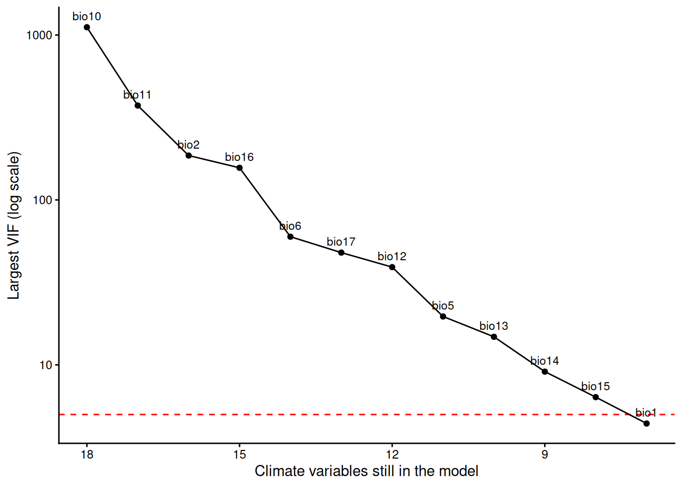
26) Sampling effort: a control we keep
Some places are surveyed far more than others. effort is the number of plant records of any species in the same pixel, log10. We know sampling effort matters for records like these, so it goes in every model, chosen before looking.
p_eff <- ggplot(pis, aes(effort, y)) +
  geom_jitter(height = 0.03, width = 0, alpha = 0.05, colour = "grey40") +
  labs(x = "Plant records in the same pixel, all species (log10)", y = "P(P. terebinthus)") +
  theme_classic()
p_eff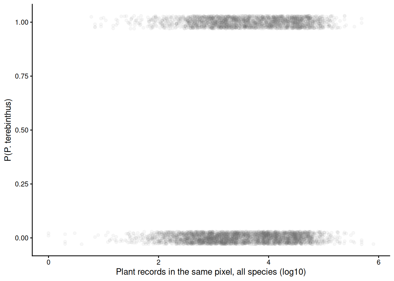
m_eff <- glm(y ~ effort, family = binomial, data = pis)
round(summary(m_eff)$coefficients, 3)
Estimate Std. Error z value Pr(>|z|)
(Intercept) -1.084 0.112 -9.691 0
effort 0.209 0.030 6.870 0ci_eff <- fit_ci(m_eff, data.frame(effort = seq(min(pis$effort), max(pis$effort), length.out = 200)))
p_eff +
geom_ribbon(data = ci_eff, aes(effort, ymin = lwr, ymax = upr), inherit.aes = FALSE, fill = "blue", alpha = 0.25) +
geom_line(data = ci_eff, aes(effort, fit), colour = "blue", linewidth = 1)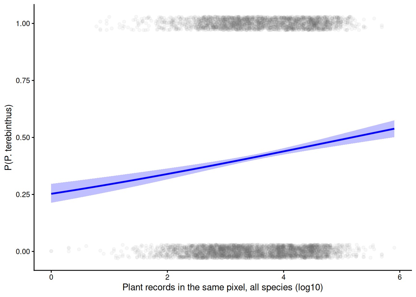
27) dredge(): fit every subset
dredge() fits every subset of the predictors in a full model and ranks them by AICc. It refuses to run unless missing values cause an error (the same-rows rule, enforced), and fixed = ~ effort keeps effort in every model: 2^7 = 128 models.
options(na.action = "na.fail")     # dredge() insists
full <- glm(y ~ bio1 + bio3 + bio4 + bio8 + bio9 + bio18 + bio19 + effort,
            family = binomial, data = pis)
dd <- dredge(full, fixed = ~ effort)   # effort in every model
nrow(dd)
[1] 12828) The top 10 of 128
The top model has six of the seven (not bio9), with only 37% of the weight, and 3 models are within 2 AICc of it. No single model is the answer. (Printing a few rows of a dredge() table rescales their weights to add to 1; recalc.weights = FALSE keeps the weights from all 128.)
dd[1:10, recalc.weights = FALSE] # keep the weights from all 128Global model call: glm(formula = y ~ bio1 + bio3 + bio4 + bio8 + bio9 + bio18 +
bio19 + effort, family = binomial, data = pis)
---
Model selection table
(Intrc) bio1 bio18 bio19 bio3 bio4 bio8 bio9 effrt df
64 -1.370 -0.4959 -0.1209 0.1866 0.06835 0.4954 -0.1490 0.2740 8
128 -1.364 -0.5161 -0.1100 0.1874 0.07212 0.4973 -0.1374 0.03419 0.2724 9
56 -1.438 -0.4977 -0.1430 0.1797 0.4788 -0.1550 0.2928 7
120 -1.437 -0.5123 -0.1360 0.1800 0.4795 -0.1468 0.02467 0.2924 8
62 -1.331 -0.3922 0.1575 0.08723 0.4982 -0.2079 0.2637 7
126 -1.328 -0.4391 0.1629 0.09054 0.5008 -0.1810 0.05443 0.2626 8
54 -1.411 -0.3690 0.1408 0.4760 -0.2303 0.2860 6
118 -1.412 -0.4096 0.1451 0.4776 -0.2074 0.04796 0.2859 7
96 -1.339 -0.6452 -0.1831 0.2511 0.08368 0.5170 0.06962 0.2651 8
32 -1.347 -0.6247 -0.2213 0.2611 0.07726 0.5166 0.2673 7
logLik AICc delta weight
64 -3898.552 7813.1 0.00 0.374
128 -3898.201 7814.4 1.31 0.195
56 -3900.259 7814.5 1.41 0.185
120 -3900.074 7816.2 3.05 0.082
62 -3901.248 7816.5 3.39 0.069
126 -3900.307 7816.6 3.51 0.065
54 -3904.197 7820.4 7.28 0.010
118 -3903.465 7820.9 7.82 0.007
96 -3902.556 7821.1 8.01 0.007
32 -3904.150 7822.3 9.19 0.004
Models ranked by AICc(x) subset(dd, delta < 2, recalc.weights = FALSE)Global model call: glm(formula = y ~ bio1 + bio3 + bio4 + bio8 + bio9 + bio18 +
bio19 + effort, family = binomial, data = pis)
---
Model selection table
(Intrc) bio1 bio18 bio19 bio3 bio4 bio8 bio9 effrt df
64 -1.370 -0.4959 -0.1209 0.1866 0.06835 0.4954 -0.1490 0.2740 8
128 -1.364 -0.5161 -0.1100 0.1874 0.07212 0.4973 -0.1374 0.03419 0.2724 9
56 -1.438 -0.4977 -0.1430 0.1797 0.4788 -0.1550 0.2928 7
logLik AICc delta weight
64 -3898.552 7813.1 0.00 0.374
128 -3898.201 7814.4 1.31 0.195
56 -3900.259 7814.5 1.41 0.185
Models ranked by AICc(x) Demo: the tile picture, and all 128 models
x <- as.data.frame(dd)[1:10, ]
tiles <- do.call(rbind, lapply(1:10, function(i) data.frame(rank = i, var = keep, inm = !is.na(unlist(x[i, keep])))))
tiles$var <- factor(tiles$var, levels = keep)
ggplot(tiles, aes(var, rank, fill = inm)) +
  geom_tile(colour = "white", linewidth = 1) +
  scale_fill_manual(values = c(`TRUE` = "blue", `FALSE` = "grey92"), guide = "none") +
  scale_y_reverse(breaks = 1:10, labels = sprintf("%d   (delta %.2f, w %.2f)", 1:10, x$delta, x$weight)) +
  scale_x_discrete(position = "top") +
  labs(x = NULL, y = NULL) +
  theme_classic()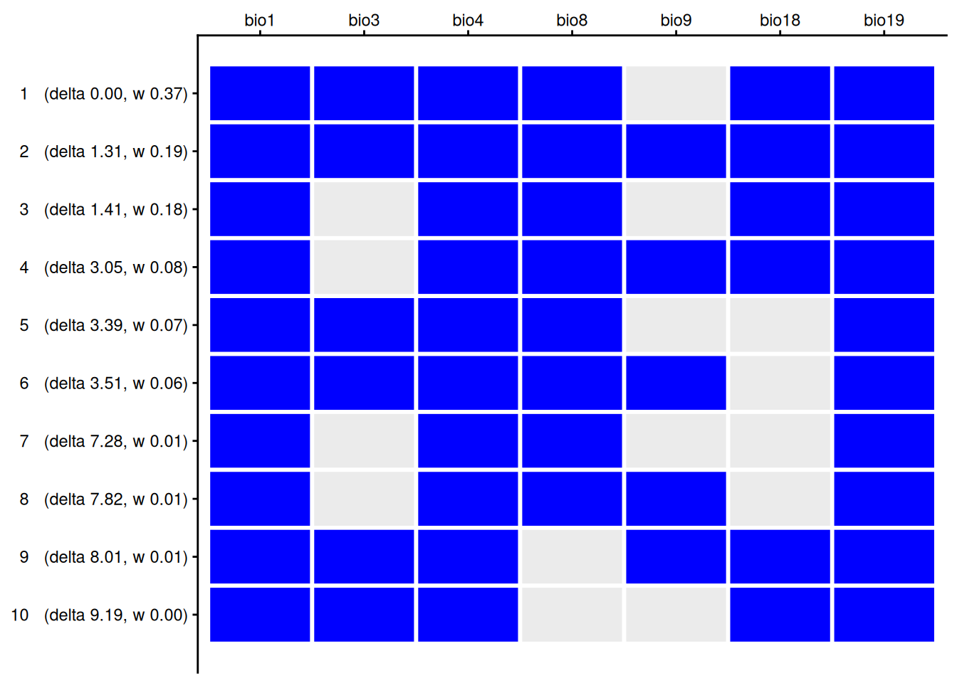
Demo: the tile picture, and all 128 models
ggplot(data.frame(rank = seq_len(nrow(dd)), delta = dd$delta), aes(rank, delta)) +
  annotate("rect", xmin = -Inf, xmax = Inf, ymin = 0, ymax = 2, fill = "green", alpha = 0.2) +
  geom_point() +
  scale_y_sqrt() +
  labs(x = "Model rank (all 128 models)", y = "Delta AICc (square-root scale)") +
  theme_classic()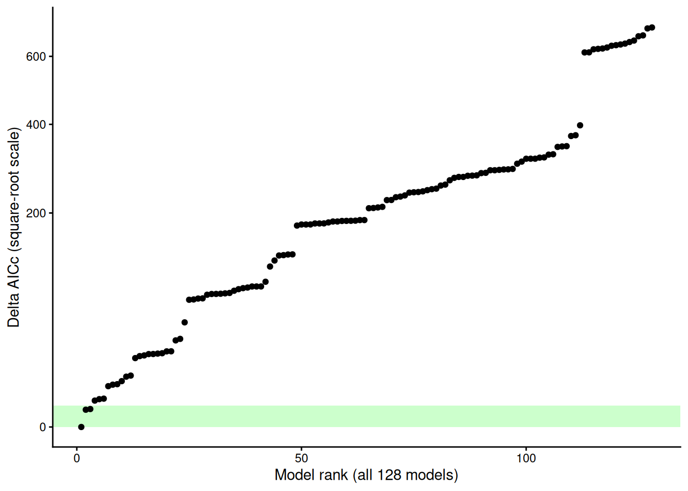
29) AICc vs BIC with 6,299 records
Ranked by BIC, the top model drops bio3 and bio18: 6 parameters instead of 8. BIC charges log(6299) = 8.7 per parameter, more than four times AIC’s 2. With large samples, AIC keeps small effects because it has the data to estimate them; BIC drops them. Say which one you used.
ddb <- dredge(full, fixed = ~ effort, rank = "BIC")
ddb[1:5, recalc.weights = FALSE]
Global model call: glm(formula = y ~ bio1 + bio3 + bio4 + bio8 + bio9 + bio18 +
bio19 + effort, family = binomial, data = pis)
---
Model selection table
(Intrc) bio1 bio18 bio19 bio3 bio4 bio8 effrt df logLik
54 -1.411 -0.3690 0.1408 0.4760 -0.2303 0.2860 6 -3904.197
56 -1.438 -0.4977 -0.1430 0.1797 0.4788 -0.1550 0.2928 7 -3900.259
62 -1.331 -0.3922 0.1575 0.08723 0.4982 -0.2079 0.2637 7 -3901.248
24 -1.425 -0.6327 -0.2514 0.2566 0.4990 0.2886 6 -3906.325
64 -1.370 -0.4959 -0.1209 0.1866 0.06835 0.4954 -0.1490 0.2740 8 -3898.552
BIC delta weight
54 7860.9 0.00 0.469
56 7861.8 0.87 0.303
62 7863.7 2.85 0.113
24 7865.1 4.26 0.056
64 7867.1 6.21 0.021
Models ranked by BIC(x) dd[1:5, recalc.weights = FALSE]Global model call: glm(formula = y ~ bio1 + bio3 + bio4 + bio8 + bio9 + bio18 +
bio19 + effort, family = binomial, data = pis)
---
Model selection table
(Intrc) bio1 bio18 bio19 bio3 bio4 bio8 bio9 effrt df
64 -1.370 -0.4959 -0.1209 0.1866 0.06835 0.4954 -0.1490 0.2740 8
128 -1.364 -0.5161 -0.1100 0.1874 0.07212 0.4973 -0.1374 0.03419 0.2724 9
56 -1.438 -0.4977 -0.1430 0.1797 0.4788 -0.1550 0.2928 7
120 -1.437 -0.5123 -0.1360 0.1800 0.4795 -0.1468 0.02467 0.2924 8
62 -1.331 -0.3922 0.1575 0.08723 0.4982 -0.2079 0.2637 7
logLik AICc delta weight
64 -3898.552 7813.1 0.00 0.374
128 -3898.201 7814.4 1.31 0.195
56 -3900.259 7814.5 1.41 0.185
120 -3900.074 7816.2 3.05 0.082
62 -3901.248 7816.5 3.39 0.069
Models ranked by AICc(x) 30) Importance: summed weights
For each variable, add up the weights of the models that contain it. With seven variables in or out, every variable is in exactly half the models, so even a useless one can collect some weight. Importance is not an effect size and not a p-value.
sw(dd) # importance: summed Akaike weights bio4 effort bio1 bio19 bio8 bio18 bio3 bio9
Sum of weights: 1.00 1.00 1.00 1.00 0.99 0.85 0.71 0.36
N containing models: 64 128 64 64 64 64 64 6431) Model averaging: estimates across the top models
Average the coefficients over the well-supported models, weighted by their Akaike weights. The full average counts a zero for a model without the variable; the conditional average uses only the models that contain it. Variables in every top model (bio1, bio4) barely change; variables in only some (bio3, bio9) are pulled toward zero.
avg <- model.avg(get.models(dd, subset = delta < 2))
summary(avg)
Call:
model.avg(object = get.models(dd, subset = delta < 2))

Component model call:
glm(formula = y ~ <3 unique rhs>, family = binomial, data = pis)

Component models:
         df   logLik    AICc delta weight
1234568   8 -3898.55 7813.13  0.00   0.50
12345678  9 -3898.20 7814.43  1.31   0.26
123568    7 -3900.26 7814.54  1.41   0.25

Term codes:
  bio1  bio18  bio19   bio3   bio4   bio8   bio9 effort
     1      2      3      4      5      6      7      8

Model-averaged coefficients:
(full average)
             Estimate Std. Error Adjusted SE z value Pr(>|z|)
(Intercept) -1.385091   0.144500    0.144526   9.584  < 2e-16 ***
bio1        -0.501584   0.059227    0.059239   8.467  < 2e-16 ***
bio18       -0.123485   0.053854    0.053864   2.293  0.02188 *
bio19        0.185113   0.037085    0.037092   4.991    6e-07 ***
bio3         0.052559   0.044063    0.044067   1.193  0.23299
bio4         0.491800   0.038545    0.038552  12.757  < 2e-16 ***
bio8        -0.147479   0.045543    0.045552   3.238  0.00121 **
effort       0.278192   0.039366    0.039374   7.065  < 2e-16 ***
bio9         0.008836   0.025596    0.025599   0.345  0.72997

(conditional average)
            Estimate Std. Error Adjusted SE z value Pr(>|z|)
(Intercept) -1.38509    0.14450     0.14453   9.584  < 2e-16 ***
bio1        -0.50158    0.05923     0.05924   8.467  < 2e-16 ***
bio18       -0.12349    0.05385     0.05386   2.293  0.02188 *
bio19        0.18511    0.03709     0.03709   4.991    6e-07 ***
bio3         0.06964    0.03719     0.03720   1.872  0.06117 .
bio4         0.49180    0.03855     0.03855  12.757  < 2e-16 ***
bio8        -0.14748    0.04554     0.04555   3.238  0.00121 **
effort       0.27819    0.03937     0.03937   7.065  < 2e-16 ***
bio9         0.03419    0.04084     0.04085   0.837  0.40262
---
Signif. codes: 0 '***' 0.001 '**' 0.01 '*' 0.05 '.' 0.1 ' ' 1round(coef(avg, full = TRUE), 2)(Intercept) bio1 bio18 bio19 bio3 bio4
-1.39 -0.50 -0.12 0.19 0.05 0.49
bio8 effort bio9
-0.15 0.28 0.01 Demo: averaged vs top-model coefficients
ct <- coefTable(avg, full = TRUE)
top <- get.models(dd, 1)[[1]]
tt <- summary(top)$coefficients
cl <- rbind(data.frame(var = rownames(ct), est = ct[, 1], se = ct[, 2], what = "averaged (delta < 2)"),
            data.frame(var = rownames(tt), est = tt[, 1], se = tt[, 2], what = "top model only"))
cl <- subset(cl, var %in% keep)
cl$var <- factor(cl$var, levels = rev(keep))
ggplot(cl, aes(est, var, colour = what)) +
  geom_vline(xintercept = 0, colour = "grey60") +
  geom_pointrange(aes(xmin = est - 1.96 * se, xmax = est + 1.96 * se), position = position_dodge(width = 0.5)) +
  scale_colour_manual(values = c("blue", "grey45"), name = NULL) +
  labs(x = "Coefficient (log odds of P. terebinthus per SD)", y = NULL) +
  theme_classic() + theme(legend.position = "bottom")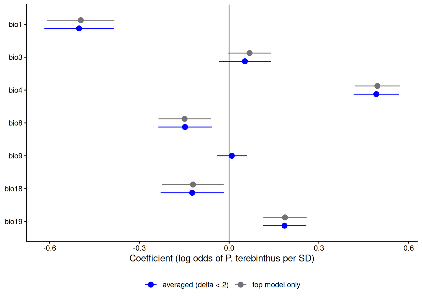
32) What we found: hypotheses, not results
The pattern from the averaged model, one variable at a time: predict over a grid of that variable with the other climate variables at their mean (0 in SD units) and effort at its mean, then put the x-axis back in raw units. The raw records go along the top and bottom.
partial_avg <- function(v) {
  nd <- data.frame(matrix(0, 150, length(keep), dimnames = list(NULL, keep)))
  nd$effort <- mean(pis$effort)
  nd[[v]] <- seq(quantile(pis[[v]], 0.01), quantile(pis[[v]], 0.99), length.out = 150)
  pr <- predict(avg, nd, se.fit = TRUE, full = TRUE)          # link (log-odds) scale
  data.frame(var = v, x = nd[[v]] * bio_sd[[v]] + bio_mean[[v]],
             fit = plogis(pr$fit), lwr = plogis(pr$fit - 1.96 * pr$se.fit), upr = plogis(pr$fit + 1.96 * pr$se.fit))
}
pe <- rbind(partial_avg("bio4"), partial_avg("bio1"))
raw_pts <- rbind(data.frame(var = "bio4", x = pis$bio4 * bio_sd[["bio4"]] + bio_mean[["bio4"]], y = pis$y),
                 data.frame(var = "bio1", x = pis$bio1 * bio_sd[["bio1"]] + bio_mean[["bio1"]], y = pis$y))
labs_v <- c(bio1 = "Annual mean temperature (bio1, °C)", bio4 = "Temperature seasonality (bio4, SD x 100)")

p_raw <- ggplot(raw_pts, aes(x, y)) +
  geom_jitter(height = 0.03, width = 0, alpha = 0.04, size = 0.6, colour = "grey40") +
  facet_wrap(~ var, scales = "free_x", labeller = as_labeller(labs_v)) +
  labs(x = NULL, y = "P(P. terebinthus)") +
  theme_classic()
p_raw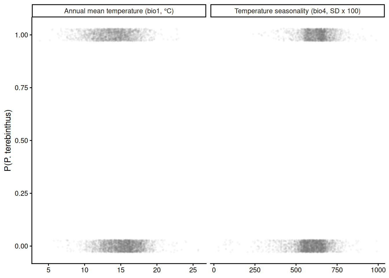
p_raw +
  geom_ribbon(data = pe, aes(x, ymin = lwr, ymax = upr), inherit.aes = FALSE, fill = "blue", alpha = 0.25) +
  geom_line(data = pe, aes(x, fit), colour = "blue", linewidth = 1)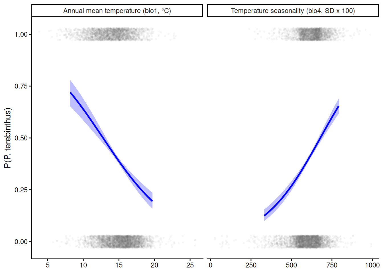
Terebinthus is more likely in cooler places with stronger seasons, which fits it being the deciduous one of the pair. But we searched 128 models for this: it is a hypothesis to test with new data, not a result.
Part E. Traps
33) Stepwise selection: drop one at a time
stepAIC() (MASS) starts from the full model and drops or adds one variable at a time while AIC improves. It visits a tiny fraction of the 32,768 models. On the cover-crop farms it keeps gdd and tmean_winter; the truth is gdd alone.
full_f <- lm(biomass ~ ., data = farms)
step_f <- stepAIC(full_f, trace = 0)     # MASS
step_f$anova                             # the path: one predictor dropped per step
Stepwise Model Path
Analysis of Deviance Table
Initial Model:
biomass ~ latitude + longitude + elevation + gdd + tmean_winter +
tmin_coldest + frost_days + rain_total + rain_wettest + rain_driest +
dry_spell + sand + silt + soil_ph + organic_matter
Final Model:
biomass ~ gdd + tmean_winter
Step Df Deviance Resid. Df Resid. Dev AIC
1 34 48838420 721.6002
2 - frost_days 1 31662.35 35 48870083 719.6326
3 - silt 1 37112.97 36 48907196 717.6706
4 - dry_spell 1 112231.50 37 49019427 715.7852
5 - tmin_coldest 1 135321.86 38 49154749 713.9231
6 - rain_total 1 534254.75 39 49689004 712.4636
7 - longitude 1 462565.38 40 50151569 710.9269
8 - rain_wettest 1 575666.83 41 50727236 709.4975
9 - elevation 1 675324.21 42 51402560 708.1588
10 - soil_ph 1 608866.72 43 52011427 706.7475
11 - organic_matter 1 950658.47 44 52962085 705.6532
12 - rain_driest 1 932905.93 45 53894991 704.5263
13 - sand 1 977325.50 46 54872317 703.4248
14 - latitude 1 1229480.55 47 56101797 702.5328attr(terms(step_f), "term.labels") # what it kept[1] "gdd" "tmean_winter"# forward: start with none, add the best one each step
step_fw <- stepAIC(lm(biomass ~ 1, data = farms), direction = "forward", trace = 0,
scope = list(lower = ~ 1, upper = reformulate(setdiff(names(farms), "biomass"))))
step_fw$anova # + gdd, + tmean_winter, stopStepwise Model Path
Analysis of Deviance Table
Initial Model:
biomass ~ 1
Final Model:
biomass ~ gdd + tmean_winter
Step Df Deviance Resid. Df Resid. Dev AIC
1 49 157802274 750.2415
2 + gdd 1 98815684 48 58986591 703.0399
3 + tmean_winter 1 2884793 47 56101797 702.532834) Resample the farms, rerun stepAIC
Resample the 50 farms with replacement 200 times (as if collecting the data again) and run stepAIC() each time. gdd is kept 99% of the time, but every one of the 14 variables that do nothing is also kept in 35% to 57.5% of the runs. The number kept ranges from 2 to 13 (median 8), and not one run finds gdd alone. (About a minute.)
Demo: stepAIC on 200 resampled data sets
set.seed(2)
sel <- replicate(200, {
  s <- farms[sample(50, 50, replace = TRUE), ]
  m <- stepAIC(lm(biomass ~ ., data = s), trace = 0)
  P %in% attr(terms(m), "term.labels")
})
rownames(sel) <- P
freq <- sort(rowMeans(sel), decreasing = TRUE)
round(freq, 3)                          # share of runs that kept each variable
gdd soil_ph latitude elevation rain_wettest
0.990 0.575 0.535 0.520 0.520
rain_driest rain_total longitude sand organic_matter
0.520 0.515 0.450 0.430 0.430
tmean_winter frost_days tmin_coldest silt dry_spell
0.425 0.425 0.415 0.400 0.350 Demo: stepAIC on 200 resampled data sets
nk <- colSums(sel)                      # predictors kept in each run
summary(nk)
Min. 1st Qu. Median Mean 3rd Qu. Max.
2.0 6.0 8.0 7.5 9.0 13.0 Demo: stepAIC on 200 resampled data sets
sum(nk == 1 & sel["gdd", ]) # runs that found the truth: gdd alone[1] 0Demo: stepAIC on 200 resampled data sets
fr <- data.frame(var = factor(names(freq), levels = rev(names(freq))), f = freq)
ggplot(fr, aes(f, var, fill = var == "gdd")) +
  geom_col(width = 0.7) +
  scale_fill_manual(values = c(`TRUE` = "blue", `FALSE` = "grey60"), guide = "none") +
  scale_x_continuous(limits = c(0, 1), labels = scales::percent) +
  labs(x = "Share of 200 resampled data sets where stepAIC() kept it", y = NULL) +
  theme_classic()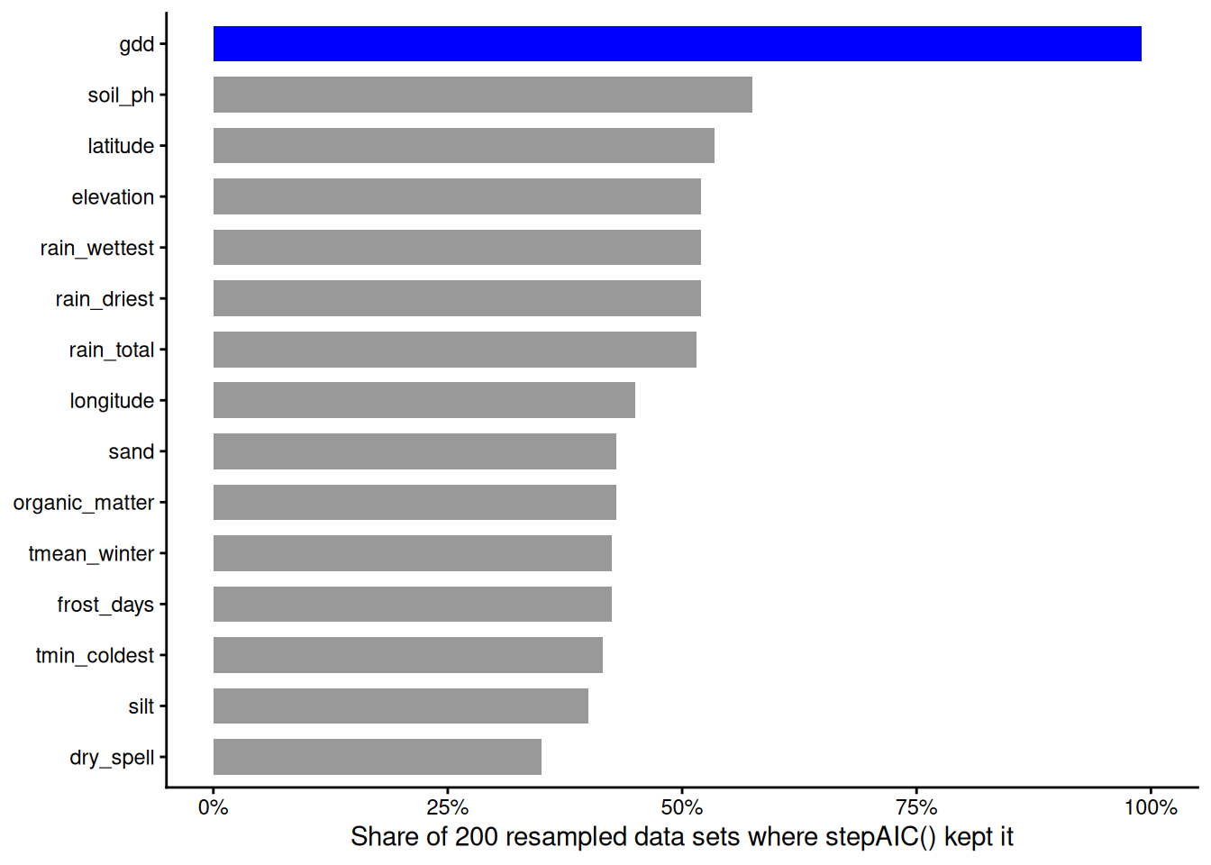
Demo: stepAIC on 200 resampled data sets
ggplot(data.frame(k = nk), aes(k)) +
  geom_bar(fill = "grey60") +
  geom_vline(xintercept = 1, colour = "blue", linewidth = 1) +
  scale_x_continuous(breaks = 0:15, limits = c(0, 15.5)) +
  labs(x = "Predictors stepAIC() kept (the truth: 1)", y = "Resampled data sets") +
  theme_classic()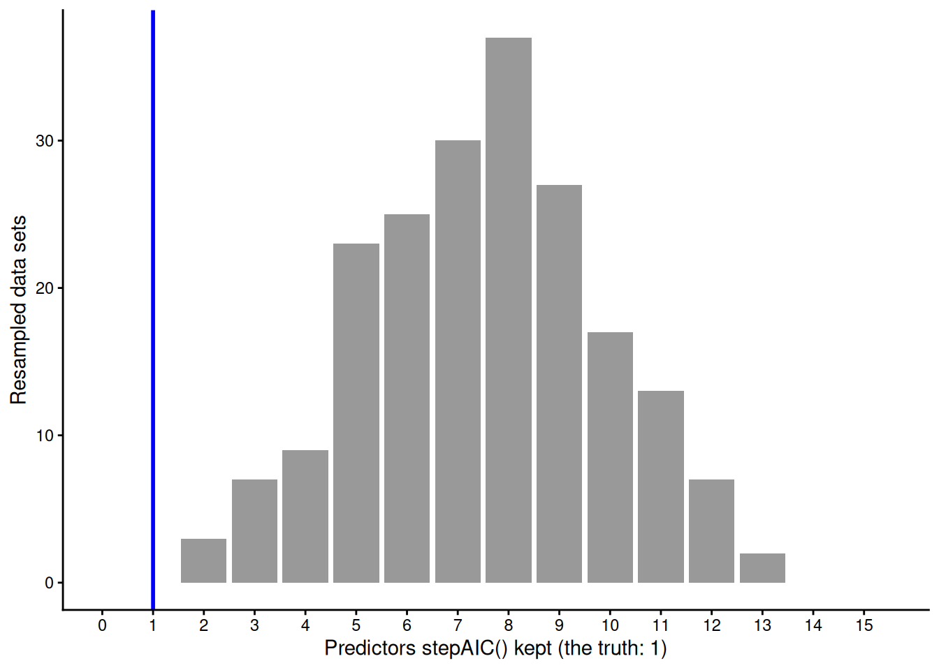
35) Pure noise, ‘significant’ results
100 rows, a response and 20 predictors, all random numbers. Stepwise keeps 5 of the 20, two of them with p = 0.006 and 0.001. The p-values are wrong because the same data were used twice: once to choose the variables, and again to test them.
Demo: stepAIC on pure noise
set.seed(41)
noise <- data.frame(y = rnorm(100), matrix(rnorm(100 * 20), 100))
step_n <- stepAIC(lm(y ~ ., data = noise), trace = 0)
round(summary(step_n)$coefficients, 3)
Estimate Std. Error t value Pr(>|t|)
(Intercept) 0.211 0.097 2.183 0.032
X1 -0.200 0.107 -1.867 0.065
X11 -0.269 0.096 -2.813 0.006
X17 0.165 0.093 1.782 0.078
X18 0.131 0.088 1.488 0.140
X20 -0.367 0.107 -3.445 0.00136) Fix: choose on one half, test on the other
1,000 pure-noise data sets of 100 rows. Choose with stepAIC() on the first 50 rows and test on the same 50: 86% end with at least one predictor at p < 0.05. Test the chosen variables on the other 50 rows instead: 25%, about what chance gives for testing five or six variables at once. (About a minute.)
Demo: 1,000 pure-noise data sets
set.seed(1)
fz <- t(replicate(1000, {
  nz <- data.frame(y = rnorm(100), matrix(rnorm(100 * 20), 100))
  a <- nz[1:50, ]; b <- nz[51:100, ]                 # choose on a, test on b
  m <- stepAIC(lm(y ~ ., data = a), trace = 0)
  tl <- attr(terms(m), "term.labels")
  same <- if (length(tl)) any(summary(m)$coefficients[-1, 4] < 0.05) else FALSE
  conf <- if (length(tl)) any(summary(lm(reformulate(tl, "y"), data = b))$coefficients[-1, 4] < 0.05) else FALSE
  c(same = same, conf = conf, k = length(tl))
}))
100 * colMeans(fz[, c("same", "conf")])   # % with a 'significant' predictor
same conf
85.6 24.6 Demo: 1,000 pure-noise data sets
mean(fz[, "k"]) # predictors kept, on average[1] 5.594Demo: 1,000 pure-noise data sets
nb <- data.frame(what = c("chosen and tested\non the same 50 rows", "chosen on 50 rows,\ntested on the other 50"),
                 pct = colMeans(fz[, c("same", "conf")]))
nb$what <- factor(nb$what, levels = nb$what)
ggplot(nb, aes(what, pct)) +
  geom_col(fill = c("red", "darkgreen"), width = 0.5) +
  geom_text(aes(label = scales::percent(pct, accuracy = 1)), vjust = -0.4) +
  scale_y_continuous(limits = c(0, 1), labels = scales::percent) +
  labs(x = NULL, y = "Data sets with a 'significant' predictor") +
  theme_classic()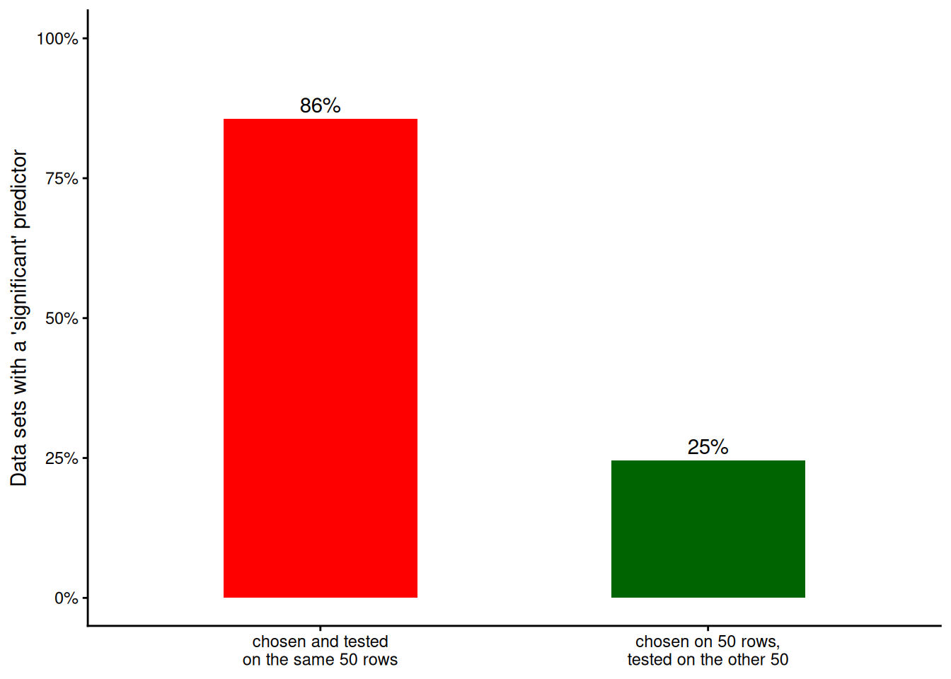
37) Selection finds predictors, not causes
Latitude alone beats the null by 6.9 AICc (97% of the weight). In the simulation latitude does nothing directly: farms further north have fewer degree days, and degree days drive biomass. AIC rewards whatever predicts, not what causes.
m_lat <- lm(biomass ~ latitude, data = farms)
round(as.data.frame(model.sel(m_null, m_lat))[, c("df", "AICc", "delta", "weight")], 3)
df AICc delta weight
m_lat 3 887.453 0.000 0.97
m_null 2 894.391 6.938 0.03g_lat <- data.frame(latitude = seq(min(farms$latitude), max(farms$latitude), length.out = 100))
ci_lat <- fit_ci(m_lat, g_lat)
p_lat <- ggplot(farms, aes(latitude, biomass / 1000)) +
geom_point(colour = "grey50") +
labs(x = "Latitude (°N)", y = "Biomass (t/ha)") +
theme_classic()
p_lat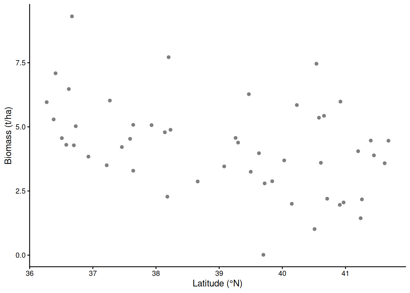
p_lat +
  geom_ribbon(data = ci_lat, aes(latitude, ymin = lwr / 1000, ymax = upr / 1000), inherit.aes = FALSE, fill = "blue", alpha = 0.2) +
  geom_line(data = ci_lat, aes(latitude, fit / 1000), colour = "blue", linewidth = 1)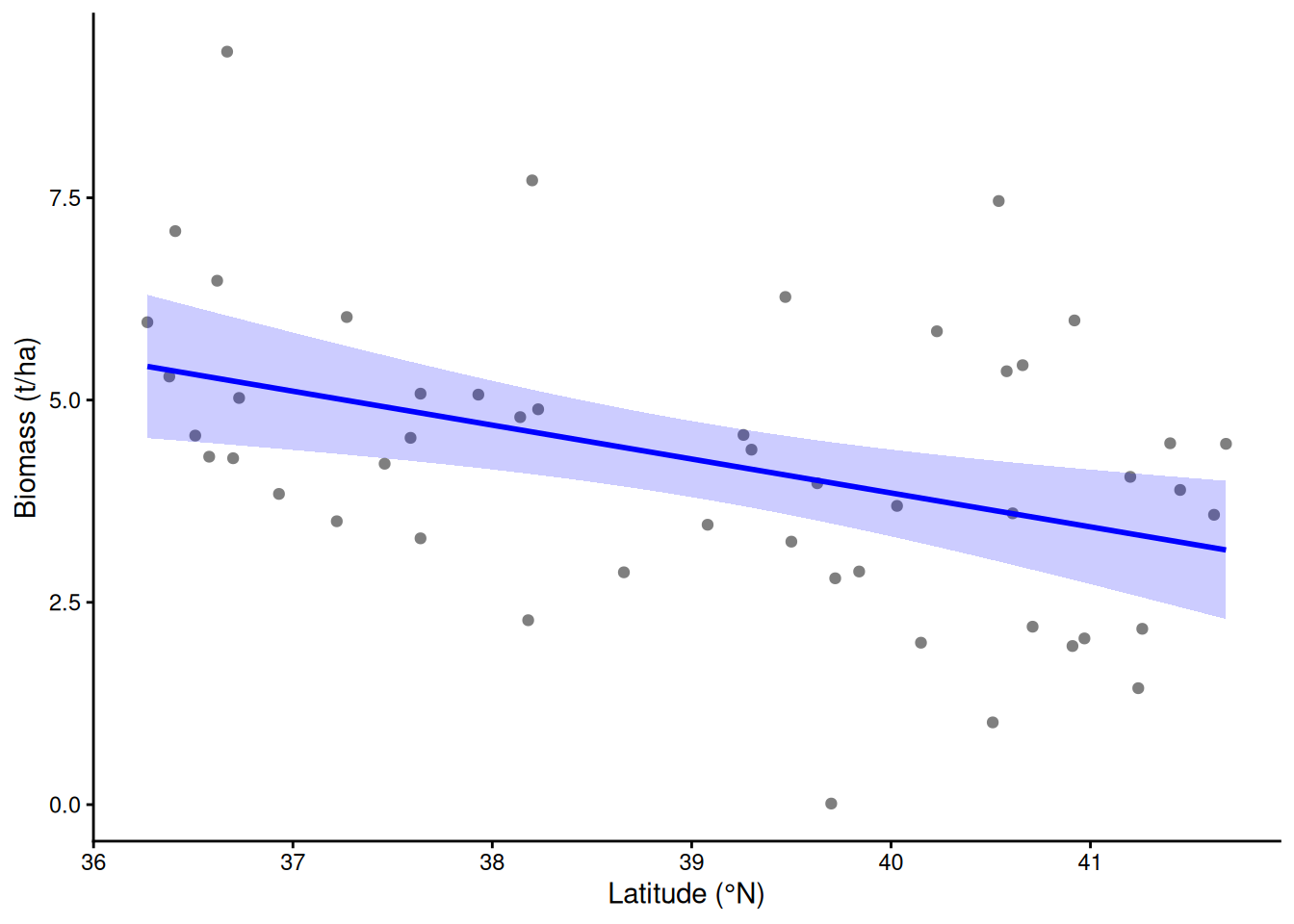
cor(farms$latitude, farms$gdd) # the path: latitude -> degree days -> biomass[1] -0.6242745Part F. Predicting
38) AIC approximates leave-one-out prediction
AIC was designed to estimate how well a model will predict new data; for large samples it behaves like leave-one-out cross-validation (fit to all but one farm, predict that farm, repeat for every farm). For a linear model the leave-one-out residual is resid / (1 - hatvalue), no refitting needed (computed in section 9). On the cover-crop sequence both curves bottom out at 2 predictors.
Demo: AIC vs leave-one-out error
fp$k[which.min(fp$loo)][1] 2Demo: AIC vs leave-one-out error
al <- rbind(data.frame(k = fp$k, v = (fp$aic - min(fp$aic)) / diff(range(fp$aic)), what = "AIC"),
            data.frame(k = fp$k, v = (fp$loo - min(fp$loo)) / diff(range(fp$loo)), what = "leave-one-out prediction error"))
ggplot(al, aes(k, v, colour = what)) +
  geom_line(linewidth = 1) + geom_point(size = 2) +
  scale_colour_manual(values = c("black", "red"), name = NULL) +
  labs(x = "Number of predictors (cover-crop farms)", y = "Scaled to 0-1") +
  theme_classic()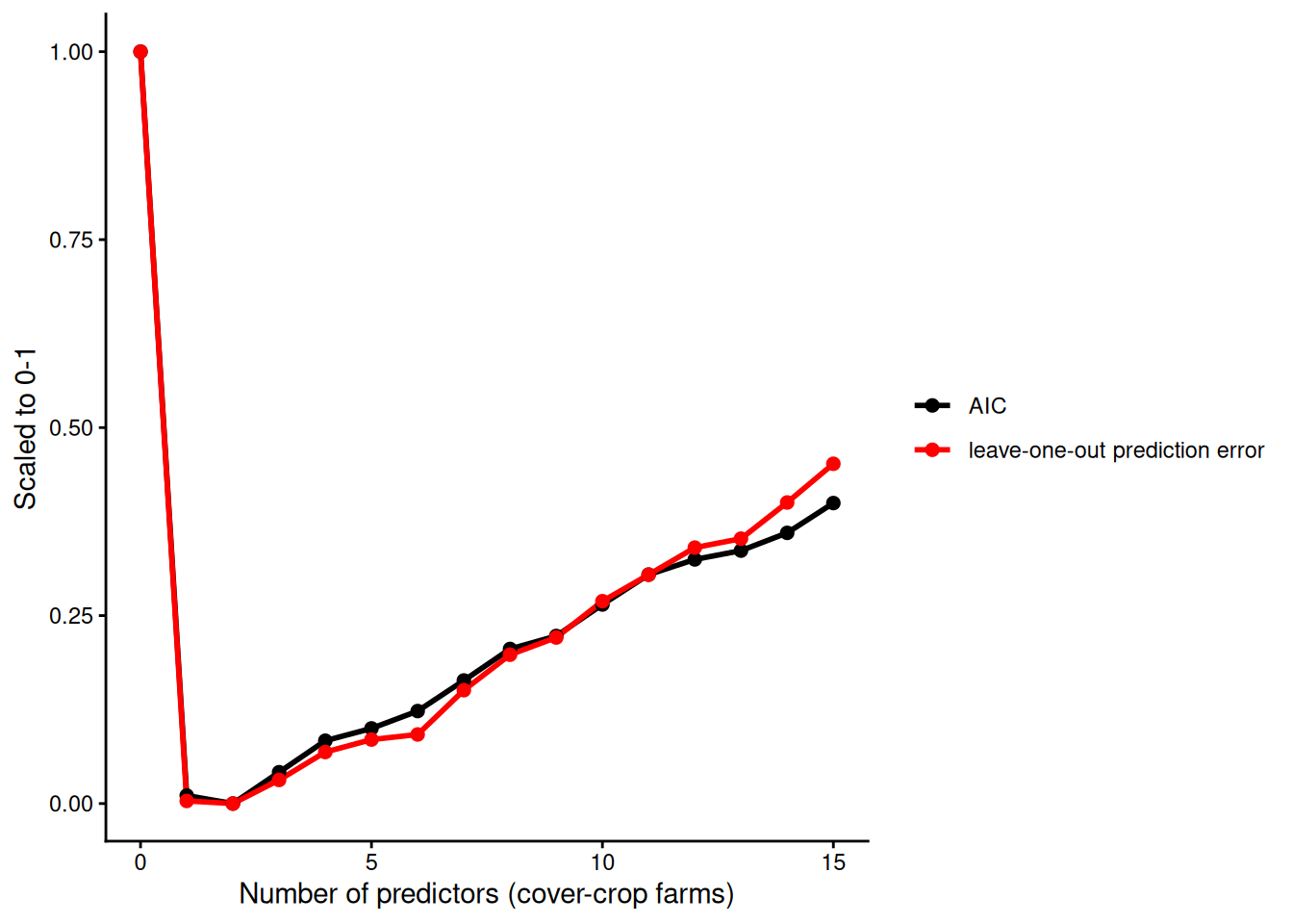
39) Next week: shrink instead of choose
Selection treats every predictor as fully in or fully out. Week 6 keeps them all and shrinks their slopes toward zero (ridge and lasso), choosing how hard to shrink by cross-validation. The lasso shrinks some slopes to exactly zero, so it selects too.
The week on one line each:
| Goal | Do |
|---|---|
| Test ideas | write the models first; model.sel(); report the table |
| Explore | dredge(); the results are hypotheses |
| Predict | held-out data, cross-validation |
| Always | the same rows and the same response; keep design terms and controls |
| Avoid | stepwise; p-values after selection |