Bonus: the GLM family

PLS 206 — seven kinds of response, one recipe

Author

Grey Monroe

The code behind the bonus deck (slides, PDF). One dataset, one predictor, seven kinds of response, and the GLM that fits each one. The interactive page lets you change the family and the coefficients and watch both scales.

GLM_families.R: the plain script. Each block is tagged [CORE], [HANDY], or [DEMO] in a comment.
GLM_families.qmd: this page as a Quarto notebook.

Every block of code on this page carries one of three labels:

Core The analysis. Code you would run on your own data: fit the model, read the output, check the diagnostics, report it. Start here for the problem sets.
Handy Useful, not essential. Wrangling, plotting, and small helpers that make the core easier. Worth knowing; skip on a first read.
Demo For the lecture only. Simulated data, sums done by hand, and the code behind slide figures. It shows why the core works. Folded: click to open.

# install.packages(c("ggplot2", "MASS"))
library(ggplot2)
library(MASS)

Every GLM is three choices:

1. distribution	what kind of number $y$ is, and how it scatters around its mean	Normal, Binomial, Poisson, negative binomial, Gamma
2. linear predictor	the same straight-line formula as `lm()`	$\eta = \beta_0 + \beta_1 x_1 + \beta_2 x_2 + \dots$
3. link	connects the mean of $y$ to the line	$g(\mu) = \eta$, so $\mu = g^{-1}(\eta)$

1) The data: seven responses, one predictor

120 wheat fields, each with one nitrogen rate (kg N/ha). Seven responses measured on every field (simulated):

column	what it is	kind of number
`yield`	grain yield, t/ha	continuous
`lodged`	crop fell over: 1 = yes, 0 = no	0/1
`sown`, `emerged`	seeds sown in a row, seedlings that emerged	$k$ of $n$
`beetles`	ground beetles in one pitfall trap, 7 days	count, same effort everywhere
`aphids`	aphids on 10 tillers	clumped count
`leaves`, `lesions`	leaves scored, septoria lesions on them	count, effort differs
`weed_biomass`	g/m²	positive, right-skewed

survey <- read.csv("https://greymonroe.github.io/PLS_206/data/field_survey.csv")
head(survey)

  field nitrogen yield lodged sown emerged beetles aphids leaves lesions
1     1      102  5.08      0  110      80       7      8     21      10
2     2      167  4.95      0  110      65       4     35     31      24
3     3      179  5.50      1  100      48       0      2     36      19
4     4       89  4.21      0  110      79       4     18     20       7
5     5       60  3.93      0   70      54       6      3     12       1
6     6       16  1.89      0   90      75       9      7     10       4
  weed_biomass
1          2.3
2         29.4
3        149.0
4         49.5
5         50.4
6         13.4

Demo: the seven responses against nitrogen

long <- rbind(
  data.frame(response = "yield (t/ha)",         nitrogen = survey$nitrogen, y = survey$yield),
  data.frame(response = "lodged (0/1)",         nitrogen = survey$nitrogen, y = survey$lodged),
  data.frame(response = "emerged / sown",       nitrogen = survey$nitrogen, y = survey$emerged / survey$sown),
  data.frame(response = "beetles per trap",     nitrogen = survey$nitrogen, y = survey$beetles),
  data.frame(response = "aphids per 10 tillers", nitrogen = survey$nitrogen, y = survey$aphids),
  data.frame(response = "lesions per leaf",     nitrogen = survey$nitrogen, y = survey$lesions / survey$leaves),
  data.frame(response = "weed biomass (g/m2)",  nitrogen = survey$nitrogen, y = survey$weed_biomass))
long$response <- factor(long$response, unique(long$response))
ggplot(long, aes(nitrogen, y)) +
  geom_point(colour = "#3D7BEB", alpha = 0.6) +
  facet_wrap(~ response, scales = "free_y", nrow = 2) +
  theme_classic()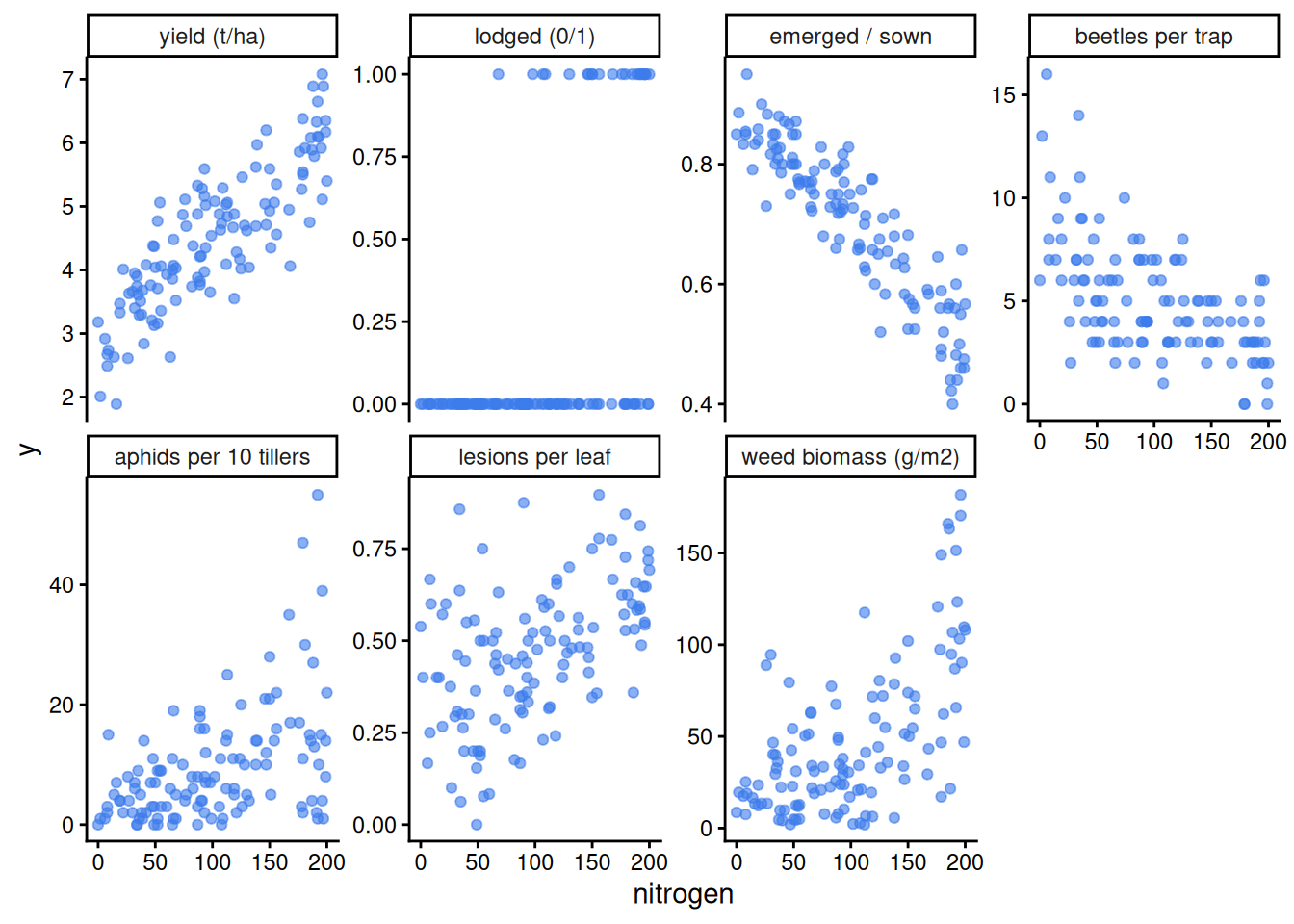

2) The link: keep the mean where it can live

A straight line runs from $-\infty$ to $+\infty$. The inverse link bends it into a range the mean can actually take. The link models the log (or logit) of the mean; it never transforms the data.

Demo: identity, log, and logit, drawn

eta <- seq(-4, 4, 0.05)
links <- rbind(data.frame(link = "identity: mu = eta",            eta, mu = eta),
               data.frame(link = "log: mu = exp(eta)",            eta, mu = exp(eta)),
               data.frame(link = "logit: mu = plogis(eta)",       eta, mu = plogis(eta)))
ggplot(links, aes(eta, mu)) +
  geom_line(colour = "#E0524A", linewidth = 1.2) +
  facet_wrap(~ link, scales = "free_y") +
  labs(x = "eta (the straight line)", y = "mu (the mean of y)") +
  theme_classic()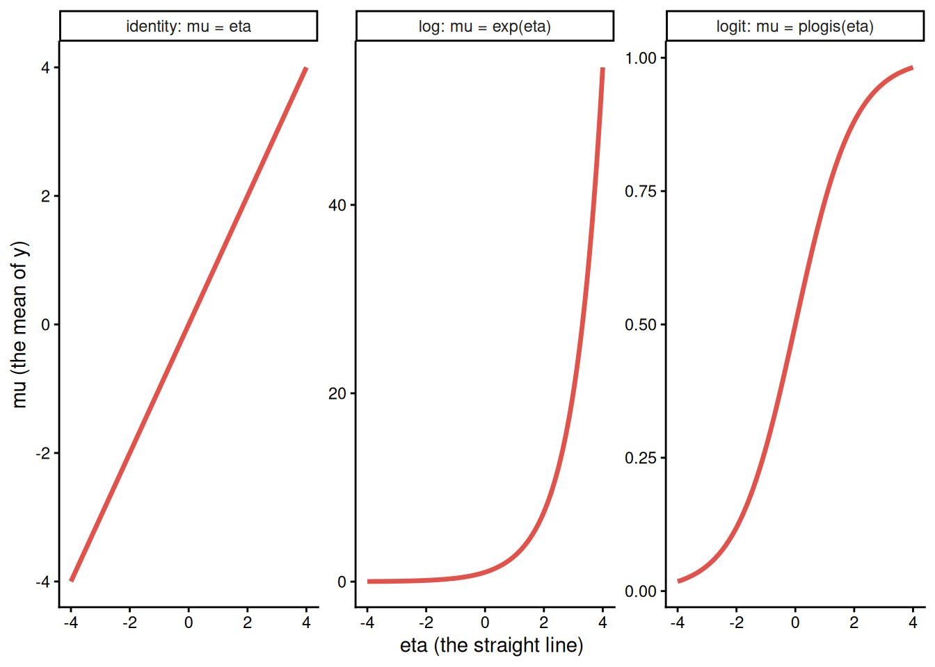

family(model)$linkfun and family(model)$linkinv hold the two directions for any fitted model; plogis() and exp() are the inverse links you will use most.

binomial()$linkfun(0.8)   # logit: log(0.8 / 0.2)

[1] 1.386294

binomial()$linkinv(1.39)  # back to a probability, same as plogis(1.39)

[1] 0.8005922

poisson()$linkinv(2)      # exp(2)

[1] 7.389056

3) The family: how spread grows with the mean

The second choice. Each family says how the variance depends on the mean: Normal $\sigma^2$ (constant), Poisson $\mu$, negative binomial $\mu + \mu^2/\theta$, Gamma $\mu^2/k$ (constant CV), binomial $p(1-p)/n$ for a proportion.

Demo: same rising mean, five families

set.seed(5)
x <- runif(400, 0, 10)
mv <- rbind(
  data.frame(family = "Normal",            x, y = rnorm(400, 2 + 1.6 * x, 2.5)),
  data.frame(family = "Poisson",           x, y = rpois(400, exp(0.5 + 0.28 * x))),
  data.frame(family = "negative binomial", x, y = rnbinom(400, mu = exp(0.5 + 0.28 * x), size = 2)),
  data.frame(family = "Gamma",             x, y = rgamma(400, shape = 3, rate = 3 / exp(0.5 + 0.28 * x))),
  data.frame(family = "binomial (k of 20)", x, y = rbinom(400, 20, plogis(-4 + 0.8 * x)) / 20))
mv$family <- factor(mv$family, unique(mv$family))
ggplot(mv, aes(x, y)) +
  geom_point(colour = "#3D7BEB", alpha = 0.4, size = 1) +
  facet_wrap(~ family, nrow = 1, scales = "free_y") +
  theme_classic()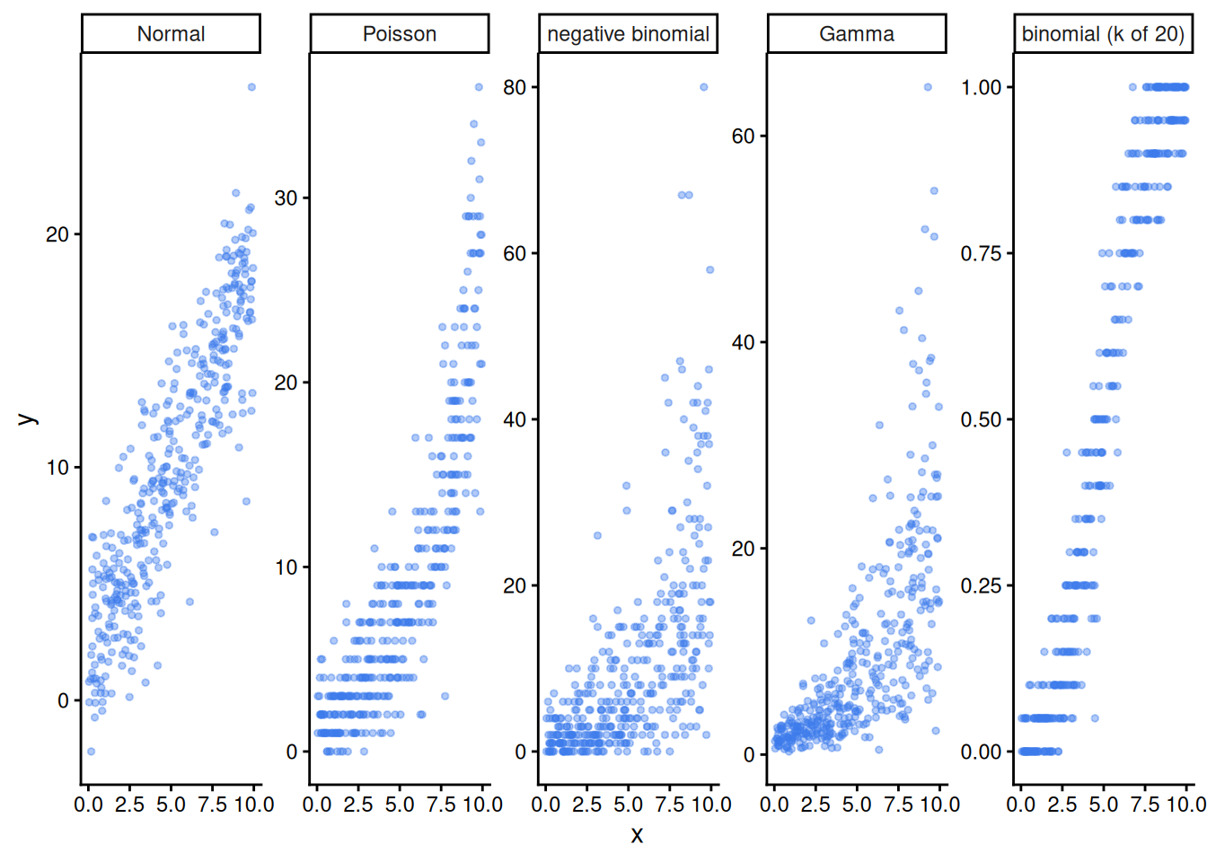

The seven models

Every section has the same shape: fit, read the coefficients, turn $\beta_1$ into a statement in the response’s own terms. Nitrogen runs 0 to 200, so the effects are reported per 100 kg N.

4) Normal: yield

$\text{yield} \sim \text{Normal}(\mu, \sigma^2)$, $\mu = \beta_0 + \beta_1\,\text{N}$. lm() is this GLM: glm(family = gaussian) gives the same estimates.

m1 <- glm(yield ~ nitrogen, family = gaussian, data = survey)
coef(summary(m1))

             Estimate   Std. Error  t value     Pr(>|t|)
(Intercept) 2.9308407 0.1073437827 27.30331 7.922147e-53
nitrogen    0.0156731 0.0009275542 16.89723 2.716035e-33

coef(lm(yield ~ nitrogen, data = survey))   # identical

(Intercept)    nitrogen 
  2.9308407   0.0156731

100 * coef(m1)["nitrogen"]                  # t/ha per 100 kg N

nitrogen 
 1.56731

5) Binomial, 0/1: did the crop lodge?

$\text{lodged} \sim \text{Bernoulli}(p)$, $\log\frac{p}{1-p} = \beta_0 + \beta_1\,\text{N}$. $e^{\beta_1}$ is an odds ratio.

m2 <- glm(lodged ~ nitrogen, family = binomial, data = survey)
coef(summary(m2))

               Estimate  Std. Error   z value     Pr(>|z|)
(Intercept) -5.22043380 0.974492412 -5.357080 8.457768e-08
nitrogen     0.02981359 0.006350583  4.694622 2.670995e-06

exp(coef(m2)["nitrogen"] * 100)                    # odds ratio, per 100 kg N

nitrogen 
19.71459

exp(confint(m2)["nitrogen", ] * 100)               # its 95% CI

    2.5 %    97.5 % 
 6.373509 79.044255

predict(m2, data.frame(nitrogen = c(50, 150)), type = "response")   # probabilities

         1          2 
0.02343629 0.32117102

6) Binomial, $k$ of $n$: seedlings emerged out of seeds sown

$\text{emerged} \sim \text{Binomial}(\text{sown}, p)$, same logit link. Put cbind(successes, failures) on the left, so a row with 120 seeds weighs more than a row with 40.

m3 <- glm(cbind(emerged, sown - emerged) ~ nitrogen, family = binomial, data = survey)
coef(summary(m3))

                Estimate   Std. Error   z value      Pr(>|z|)
(Intercept)  1.876734509 0.0500493886  37.49765 1.005943e-307
nitrogen    -0.009483404 0.0003892029 -24.36622 3.902679e-131

exp(coef(m3)["nitrogen"] * 100)   # odds ratio, per 100 kg N

 nitrogen 
0.3873834

The same model, written as a proportion with weights:

m3b <- glm(emerged / sown ~ nitrogen, family = binomial, weights = sown, data = survey)
coef(m3b)

 (Intercept)     nitrogen 
 1.876734509 -0.009483404

7) Poisson: beetles per trap

$\text{beetles} \sim \text{Poisson}(\mu)$, $\log\mu = \beta_0 + \beta_1\,\text{N}$. $e^{\beta_1}$ is a rate ratio. Every field had the same effort (one trap, one week).

m4 <- glm(beetles ~ nitrogen, family = poisson, data = survey)
coef(summary(m4))

                Estimate   Std. Error   z value      Pr(>|z|)
(Intercept)  2.125287480 0.0729219240 29.144698 9.751810e-187
nitrogen    -0.005702565 0.0007423705 -7.681562  1.571607e-14

exp(coef(m4)["nitrogen"] * 100)        # rate ratio, per 100 kg N

 nitrogen 
0.5653804

deviance(m4) / df.residual(m4)         # about 1: Poisson spread fits

[1] 0.9770481

8) Overdispersion: is Poisson enough for the aphids?

Poisson forces variance = mean. Residual deviance / df well above 1 means the counts are more spread out than that, and the Poisson standard errors are too small.

m5p <- glm(aphids ~ nitrogen, family = poisson, data = survey)
deviance(m5p) / df.residual(m5p)

[1] 5.934917

Demo: the Poisson 95% band is far too narrow for the aphids

g <- data.frame(nitrogen = 0:200)
g$mu <- predict(m5p, g, type = "response")
g$lo <- qpois(0.025, g$mu); g$hi <- qpois(0.975, g$mu)
ggplot(survey, aes(nitrogen, aphids)) +
  geom_ribbon(data = g, aes(nitrogen, ymin = lo, ymax = hi), inherit.aes = FALSE, fill = "red", alpha = 0.15) +
  geom_point(colour = "#3D7BEB") +
  geom_line(data = g, aes(nitrogen, mu), colour = "red") +
  theme_classic()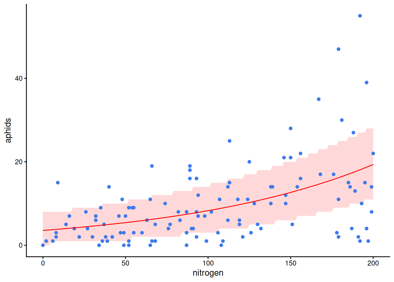

Demo: the Poisson 95% band is far too narrow for the aphids

outside <- with(survey, aphids < qpois(0.025, fitted(m5p)) | aphids > qpois(0.975, fitted(m5p)))
mean(outside)   # share of fields outside the band (should be about 0.05)

[1] 0.3666667

9) Negative binomial: aphids

$\text{aphids} \sim \text{NegBin}(\mu, \theta)$, $\log\mu = \beta_0 + \beta_1\,\text{N}$, $\text{Var} = \mu + \mu^2/\theta$. Same link and same reading of $\beta_1$ as Poisson; one more parameter for the spread.

m5 <- glm.nb(aphids ~ nitrogen, data = survey)
coef(summary(m5))

               Estimate  Std. Error  z value     Pr(>|z|)
(Intercept) 1.231085761 0.159436330 7.721488 1.149791e-14
nitrogen    0.008786187 0.001327348 6.619353 3.607748e-11

m5$theta                               # smaller = more clumped

[1] 1.702964

exp(coef(m5)["nitrogen"] * 100)        # rate ratio, per 100 kg N

nitrogen 
2.407572

# the standard error of the nitrogen slope, three ways
m5q <- glm(aphids ~ nitrogen, family = quasipoisson, data = survey)
c(poisson = coef(summary(m5p))[2, 2],
  quasipoisson = coef(summary(m5q))[2, 2],
  negbin = coef(summary(m5))[2, 2])

     poisson quasipoisson       negbin 
0.0005253985 0.0012679079 0.0013273483

10) Counts per effort: the offset

Scouts scored different numbers of leaves per field, and more on high-nitrogen fields. The question is lesions per leaf. An offset puts $\log(\text{leaves})$ in the linear predictor with its coefficient fixed at 1:

\[\log\mu = \log(\text{leaves}) + \beta_0 + \beta_1\,\text{N} \quad\Longleftrightarrow\quad \log\frac{\mu}{\text{leaves}} = \beta_0 + \beta_1\,\text{N}\]

m6 <- glm(lesions ~ nitrogen + offset(log(leaves)), family = poisson, data = survey)
coef(summary(m6))

                Estimate   Std. Error    z value     Pr(>|z|)
(Intercept) -1.162398954 0.0726126759 -16.008210 1.119857e-57
nitrogen     0.003668435 0.0005034928   7.285972 3.193588e-13

exp(coef(m6)["nitrogen"] * 100)        # lesions per leaf, ratio per 100 kg N

nitrogen 
1.443172

deviance(m6) / df.residual(m6)

[1] 1.162381

Leave the offset out and nitrogen also gets the credit for the extra leaves scored:

m6x <- glm(lesions ~ nitrogen, family = poisson, data = survey)
exp(coef(m6x)["nitrogen"] * 100)       # no offset: too steep

nitrogen 
2.735118

cor(survey$nitrogen, survey$leaves)    # because effort rises with nitrogen

[1] 0.9251543

Predictions from an offset model need the effort column. leaves = 1 gives the rate per leaf:

predict(m6, data.frame(nitrogen = c(50, 150), leaves = 1), type = "response")

        1         2 
0.3756952 0.5421927

The negative binomial takes an offset the same way: glm.nb(y ~ x + offset(log(effort))).

11) Gamma: weed biomass

Positive, continuous, right-skewed, spread growing with the mean. $\text{weeds} \sim \text{Gamma}$, $\log\mu = \beta_0 + \beta_1\,\text{N}$, $\text{Var} = \mu^2/k$.

m7 <- glm(weed_biomass ~ nitrogen, family = Gamma(link = "log"), data = survey)
coef(summary(m7))

               Estimate  Std. Error   t value     Pr(>|t|)
(Intercept) 2.898090364 0.130031201 22.287654 4.156874e-44
nitrogen    0.008254916 0.001123595  7.346875 2.867309e-11

exp(coef(m7)["nitrogen"] * 100)        # ratio of mean biomass, per 100 kg N

nitrogen 
2.283003

1 / summary(m7)$dispersion             # the shape k (about 2 in the simulation)

[1] 1.93408

The usual alternative, lm(log(y) ~ x), models the mean of $\log y$ (a geometric mean), not the mean itself, and fails on zeros:

exp(coef(lm(log(weed_biomass) ~ nitrogen, data = survey))["nitrogen"] * 100)

nitrogen 
2.530331

Reading and plotting any GLM

12) One rule per link

link	model	$x + 1$ does
identity	$\mu = \beta_0 + \beta_1 x$	adds $\beta_1$ to the mean
log	$\mu = e^{\beta_0} e^{\beta_1 x}$	multiplies the mean by $e^{\beta_1}$
logit	$\text{odds} = e^{\beta_0} e^{\beta_1 x}$	multiplies the odds by $e^{\beta_1}$

new <- data.frame(nitrogen = c(50, 150), leaves = 1)
predict(m2, new, type = "link")        # log-odds

         1          2 
-3.7297544 -0.7483955

predict(m2, new, type = "response")    # probability

         1          2 
0.02343629 0.32117102

13) The fitted curve with a confidence band, for any family

Build the band on the link scale (where it is symmetric), then back-transform.

glm_curve <- function(model, data, x = "nitrogen", ...) {
  g <- data.frame(seq(min(data[[x]]), max(data[[x]]), length.out = 200), ...)
  names(g)[1] <- x
  p <- predict(model, g, type = "link", se.fit = TRUE)
  inv <- family(model)$linkinv
  g$fit <- inv(p$fit)
  g$lo <- inv(p$fit - 1.96 * p$se.fit)
  g$hi <- inv(p$fit + 1.96 * p$se.fit)
  g
}
band <- glm_curve(m4, survey)
ggplot(survey, aes(nitrogen, beetles)) +
  geom_ribbon(data = band, aes(nitrogen, ymin = lo, ymax = hi), inherit.aes = FALSE, alpha = 0.2) +
  geom_point(colour = "#3D7BEB") +
  geom_line(data = band, aes(nitrogen, fit), colour = "red", linewidth = 1) +
  theme_classic()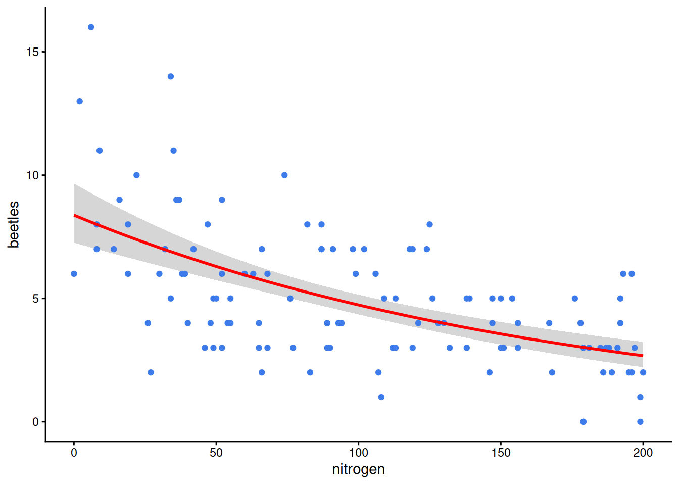

14) All seven at once

models <- list(yield = m1, lodged = m2, emerged = m3, beetles = m4,
               aphids = m5, lesions = m6, weeds = m7)
data.frame(
  family = sapply(models, function(m) family(m)$family),
  link   = sapply(models, function(m) family(m)$link),
  beta1  = sapply(models, function(m) coef(m)["nitrogen"]),
  per100 = sapply(models, function(m) {
    b <- 100 * coef(m)["nitrogen"]
    if (family(m)$link == "identity") b else exp(b)
  }),
  p = sapply(models, function(m) coef(summary(m))["nitrogen", 4]))

                          family     link        beta1     per100             p
yield                   gaussian identity  0.015673099  1.5673099  2.716035e-33
lodged                  binomial    logit  0.029813589 19.7145882  2.670995e-06
emerged                 binomial    logit -0.009483404  0.3873834 3.902679e-131
beetles                  poisson      log -0.005702565  0.5653804  1.571607e-14
aphids  Negative Binomial(1.703)      log  0.008786187  2.4075717  3.607748e-11
lesions                  poisson      log  0.003668435  1.4431720  3.193588e-13
weeds                      Gamma      log  0.008254916  2.2830028  2.867309e-11

per100 is a difference for yield (t/ha), an odds ratio for lodged and emerged, and a ratio of means for the rest.

15) Beyond these seven

response	function
ordered categories (none < mild < severe)	`MASS::polr()`
three or more unordered categories	`nnet::multinom()`
too many zeros	`glmmTMB::glmmTMB(..., ziformula = ~ 1)`
continuous proportions (% cover)	`glmmTMB::glmmTMB(..., family = beta_family())`
any of these with plots nested in farms	`lme4::glmer(..., family = ...)`

link	model	\(x + 1\) does
identity	\(\mu = \beta_0 + \beta_1 x\)	adds \(\beta_1\) to the mean
log	\(\mu = e^{\beta_0} e^{\beta_1 x}\)	multiplies the mean by \(e^{\beta_1}\)
logit	\(\text{odds} = e^{\beta_0} e^{\beta_1 x}\)	multiplies the odds by \(e^{\beta_1}\)