Week 2: Linear regression
PLS 206 — the code behind the lectures
One page for the whole week. It follows the slides (Week2_Linear_Regression.pptx) in order, and has the code behind every figure and number in the lecture, with the output underneath.
To run it yourself, download either version and open it in RStudio. It reads the data straight from the course website, so there is no file to download and no working directory to set:
- Week2_Linear_Regression.R: the plain script. Each block is tagged
[CORE],[HANDY], or[DEMO]in a comment. - Week2_Linear_Regression.qmd: this page as a Quarto notebook (open in RStudio, run chunk by chunk, or click Render).
Every block of code on this page carries one of three labels:
- Core The analysis. Code you would run on your own data: fit the model, read the output, check the diagnostics, report it. Start here for the problem sets.
- Handy Useful, not essential. Wrangling, plotting, and small helpers that make the core easier. Worth knowing; skip on a first read.
- Demo For the lecture only. Simulated data, sums done by hand, and the code behind slide figures. It shows why the core works. Folded: click to open.
# install.packages(c("ggplot2", "car", "scatterplot3d"))
library(ggplot2)
Part A. Fitting a line
1) The data: 40 wheat plants
wheat <- read.csv("https://greymonroe.github.io/PLS_206/data/wheat_plants.csv")
head(wheat)
plant water nitrogen height biomass
1 1 45 89 86.9 18.1
2 2 41 6 71.6 15.5
3 3 21 66 73.1 14.8
4 4 31 70 75.9 15.6
5 5 49 115 91.0 21.6
6 6 49 65 94.4 17.2nrow(wheat)[1] 40Always plot first.
plot(wheat$height, wheat$biomass, xlab = "Height (cm)", ylab = "Biomass (g)")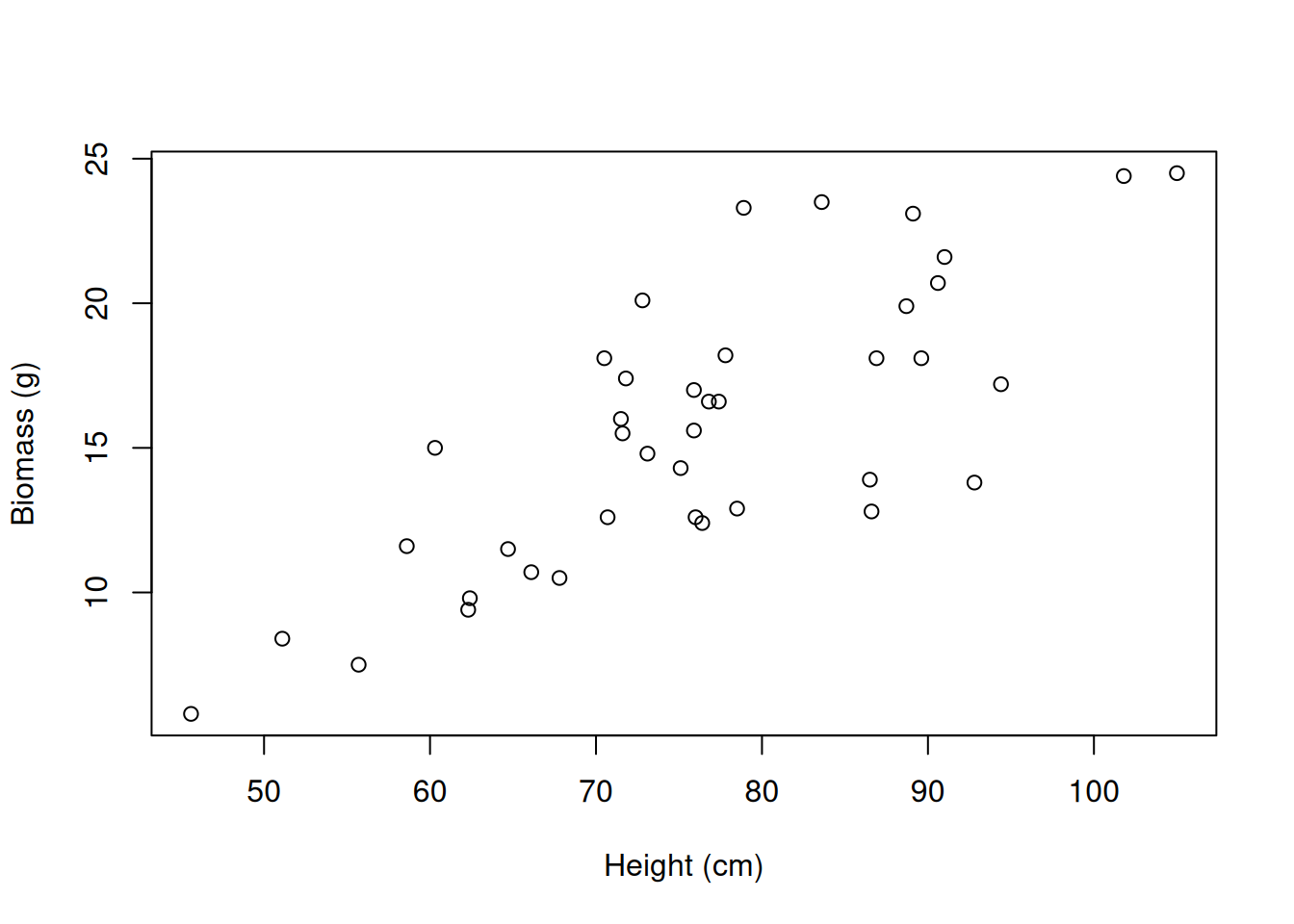
ggplot(wheat, aes(height, biomass)) +
  geom_point() +
  labs(x = "Height (cm)", y = "Biomass (g)") +
  theme_classic()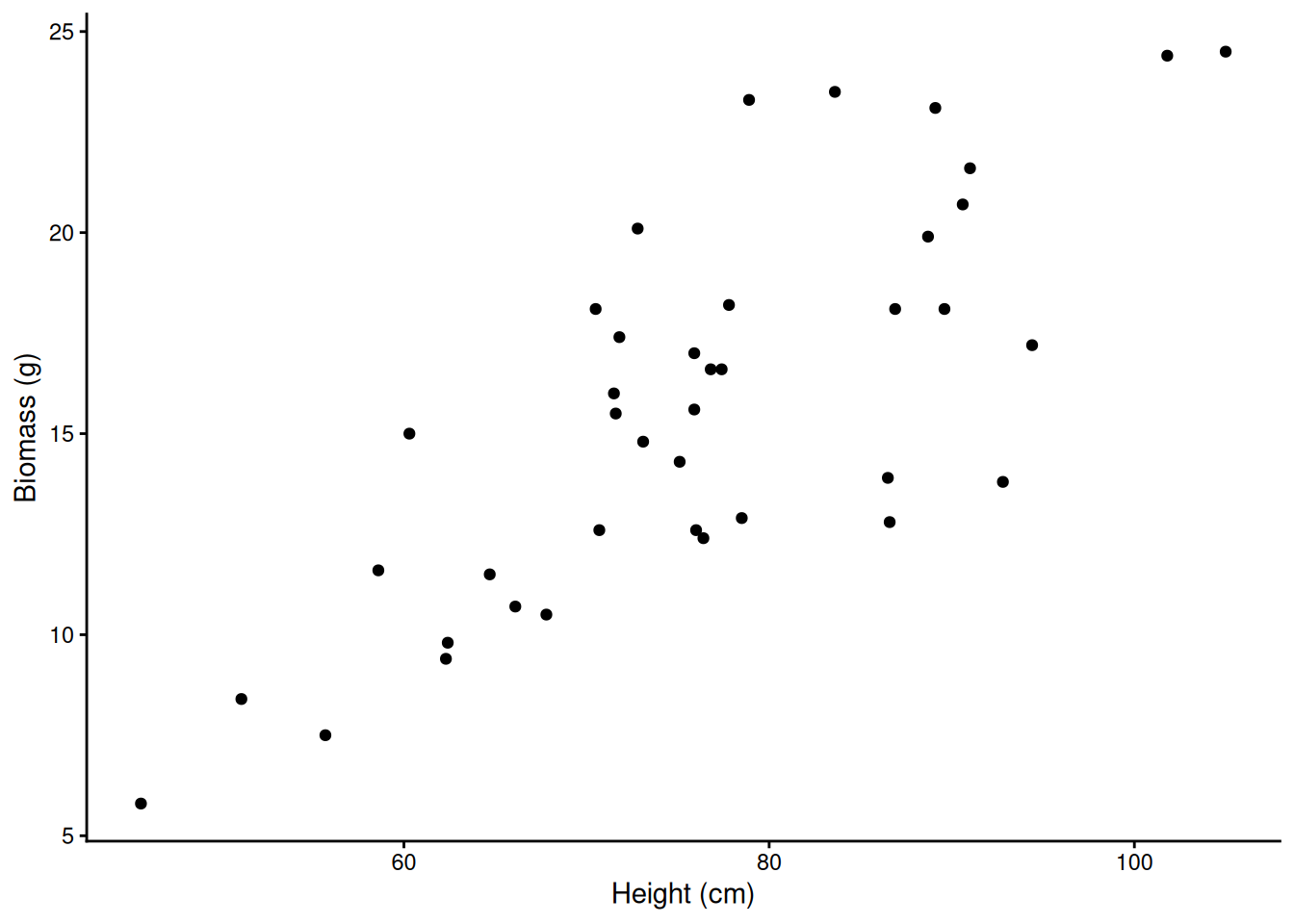
2) Scoring a line: residuals and the sum of squares
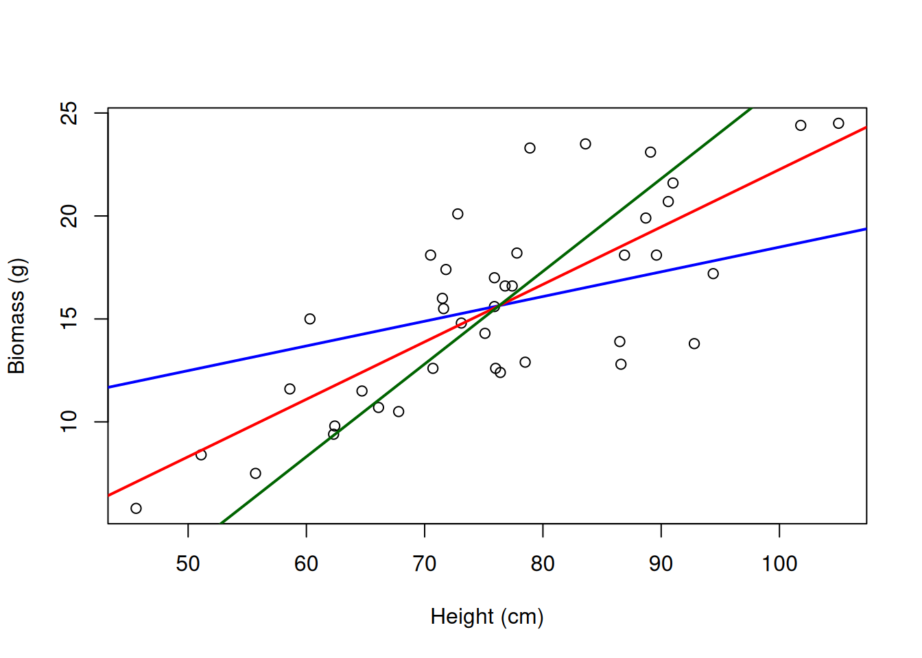
Any line through the middle of the data: biomass = b0 + slope * height. Score each candidate line by its residual sum of squares (RSS). lm() does all of this for you in section 4.
Demo: a function that scores a line by its RSS
# score a line through the middle of the data by its RSS
model_line <- function(slope) {
  b0 <- mean(wheat$biomass) - slope * mean(wheat$height)
  predicted <- b0 + slope * wheat$height
  sum((wheat$biomass - predicted)^2)
}
model_line(0.12)    # line A
[1] 533.4545Demo: a function that scores a line by its RSS
model_line(0.279) # line B[1] 361.2284Demo: a function that scores a line by its RSS
model_line(0.45) # line C[1] 560.0627Demo: the three candidate lines
# the three candidate lines on the plot (all through the middle of the data)
plot(wheat$height, wheat$biomass, xlab = "Height (cm)", ylab = "Biomass (g)")
for (slope in c(0.12, 0.279, 0.45)) {
  b0 <- mean(wheat$biomass) - slope * mean(wheat$height)
  abline(b0, slope, col = c("blue", "red", "darkgreen")[match(slope, c(0.12, 0.279, 0.45))], lwd = 2)
}
Demo: residuals from line B, and why we square them
# residuals: the vertical distance from each point to line B
b0 <- mean(wheat$biomass) - 0.279 * mean(wheat$height)
predicted <- b0 + 0.279 * wheat$height
residual  <- wheat$biomass - predicted
plot(wheat$height, wheat$biomass, xlab = "Height (cm)", ylab = "Biomass (g)")
abline(b0, 0.279, col = "red", lwd = 2)
segments(wheat$height, wheat$biomass, wheat$height, predicted, col = "blue", lty = 2)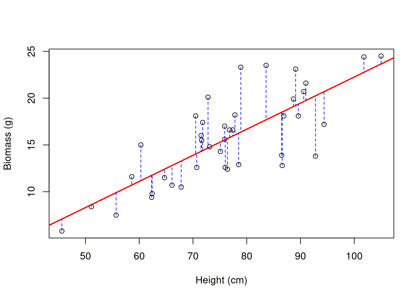
Demo: residuals from line B, and why we square them
sum(residual) # they cancel out...[1] 8.082424e-14Demo: residuals from line B, and why we square them
sum(residual^2) # ...so we square them: the residual sum of squares[1] 361.2284Demo: the RSS drawn as squares
# squares whose side is the residual: the RSS is their total area
plot(wheat$height, wheat$biomass, xlab = "Height (cm)", ylab = "Biomass (g)", asp = 1)
abline(b0, 0.279, col = "red", lwd = 2)
rect(wheat$height, pmin(wheat$biomass, predicted), wheat$height + abs(residual),
     pmax(wheat$biomass, predicted), col = adjustcolor("blue", 0.2), border = "blue")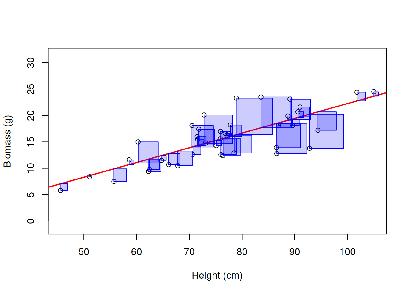
Demo: the RSS for every slope is a bowl
# the RSS for every slope from 0 to 0.6: a bowl with its bottom at 0.279
slopes <- seq(0, 0.6, by = 0.005)
rss <- sapply(slopes, model_line)
plot(slopes, rss, type = "l", xlab = "Slope (g per cm)", ylab = "Residual sum of squares")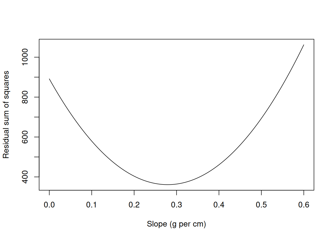
Demo: the RSS for every slope is a bowl
slopes[which.min(rss)][1] 0.28Demo: both knobs at once (intercept and slope)
# both knobs at once: the RSS over intercept and slope is a bowl
rss2 <- function(b0, b1) sum((wheat$biomass - (b0 + b1 * wheat$height))^2)
b0s <- seq(-20, 10, length.out = 60); b1s <- seq(0.1, 0.45, length.out = 60)
bowl <- outer(b0s, b1s, Vectorize(rss2))
persp(b0s, b1s, bowl, theta = 35, phi = 25, xlab = "intercept", ylab = "slope", zlab = "RSS", col = "lightblue")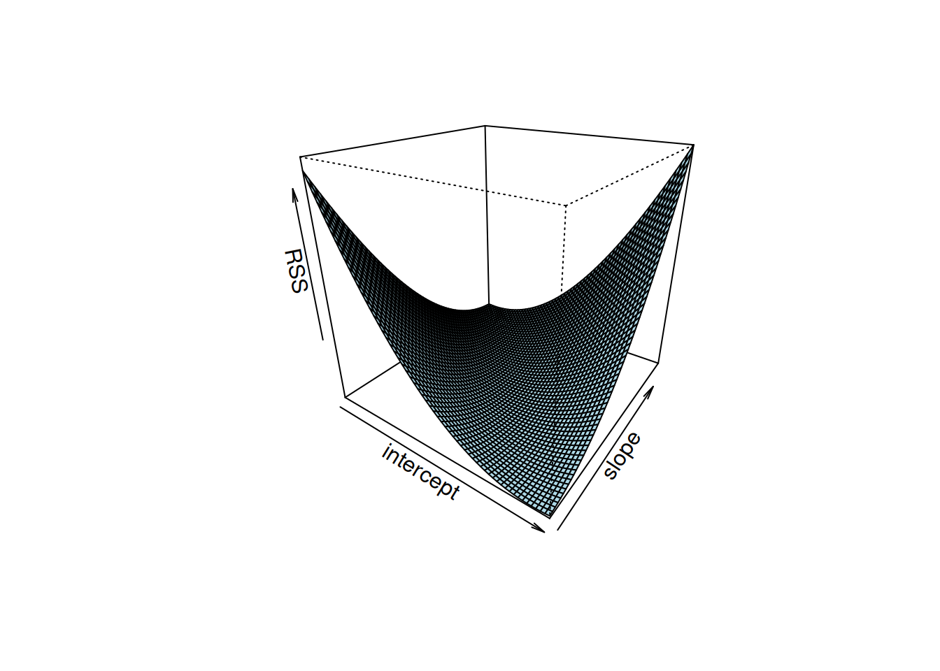
Demo: both knobs at once (intercept and slope)
# the bottom of the bowl:
c(b0s[which(bowl == min(bowl), arr.ind = TRUE)[1]], b1s[which(bowl == min(bowl), arr.ind = TRUE)[2]])
[1] -5.2542373 0.27203393) The least-squares slope and intercept by hand
Demo: slope and intercept from cov(), var(), and cor()
# slope
b1 <- cov(wheat$height, wheat$biomass) / var(wheat$height)
b1
[1] 0.2790764Demo: slope and intercept from cov(), var(), and cor()
# intercept
b0 <- mean(wheat$biomass) - b1 * mean(wheat$height)
b0
[1] -5.647833Demo: slope and intercept from cov(), var(), and cor()
# the same slope, via r
r <- cor(wheat$height, wheat$biomass)
r * sd(wheat$biomass) / sd(wheat$height)
[1] 0.27907644) lm(): the same line
# lm(response ~ predictor, data = data.frame)
model <- lm(biomass ~ height, data = wheat)
model
Call:
lm(formula = biomass ~ height, data = wheat)

Coefficients:
(Intercept)       height
-5.6478 0.2791 coef(model)(Intercept) height
-5.6478330 0.2790764 plot(wheat$height, wheat$biomass, xlab = "Height (cm)", ylab = "Biomass (g)")
abline(model, col = "red", lwd = 2)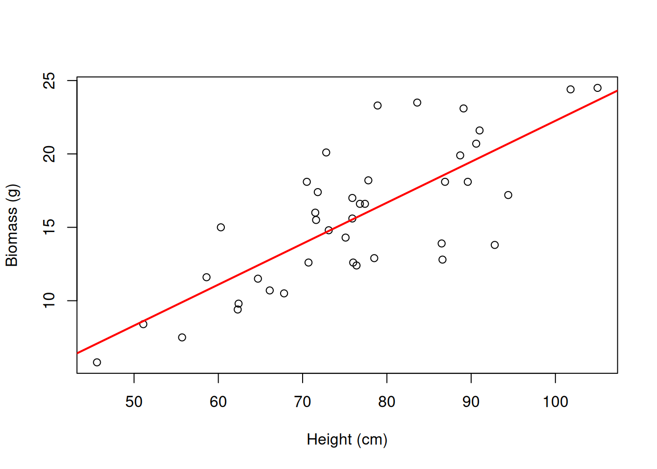
5) Predictions
predict(model, newdata = data.frame(height = 100)) 1
22.25981 -5.65 + 0.279 * 100 # the same thing from the equation[1] 22.25new <- data.frame(height = c(60, 80, 100))
predict(model, newdata = new) 1 2 3
11.09675 16.67828 22.25981 # fitted values and residuals for our own 40 plants
wheat$predicted <- predict(model) # fitted values
wheat$residual <- resid(model)
head(wheat[, c("height", "biomass", "predicted", "residual")]) height biomass predicted residual
1 86.9 18.1 18.60391 -0.50390773
2 71.6 15.5 14.33404 1.16596148
3 73.1 14.8 14.75265 0.04734685
4 75.9 15.6 15.53407 0.06593288
5 91.0 21.6 19.74812 1.85187896
6 94.4 17.2 20.69698 -3.49698087Demo: observed = predicted + residual
# observed = predicted + residual
head(wheat$predicted + wheat$residual)
[1] 18.1 15.5 14.8 15.6 21.6 17.2Demo: observed = predicted + residual
head(wheat$biomass)[1] 18.1 15.5 14.8 15.6 21.6 17.2Demo: observed = predicted + residual
sum(wheat$residual) # residuals sum to zero (up to rounding)[1] 2.629841e-15# interpolate, don't extrapolate: predict() will answer anything
predict(model, newdata = data.frame(height = c(0, 200))) # nonsense plants 1 2
-5.647833 50.167451 range(wheat$height) # where the data are[1] 45.6 105.05b) The line is a conditional mean
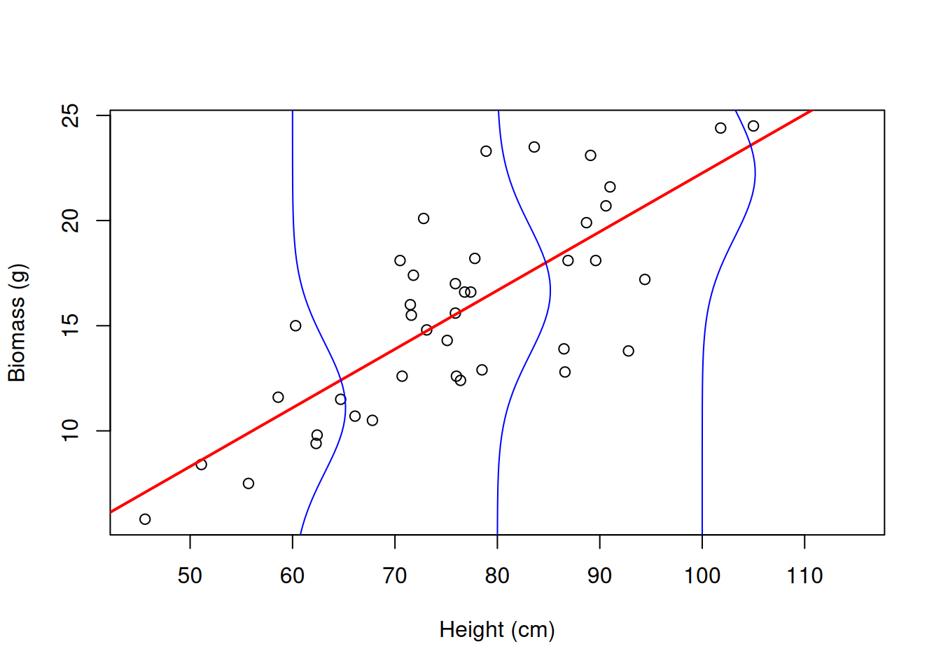
At each height, biomass is a distribution: mean on the line, spread sigma.
sigma(model) # residual standard error: the typical miss[1] 3.083182Demo: the normal curve of biomass at three heights
mu <- predict(model, data.frame(height = c(60, 80, 100)))
cbind(height = c(60, 80, 100), mean = mu, low = mu - 2 * sigma(model), high = mu + 2 * sigma(model))
height mean low high
1 60 11.09675 4.930389 17.26312
2 80 16.67828 10.511917 22.84464
3 100 22.25981 16.093445 28.42617Demo: the normal curve of biomass at three heights
# the model's assumption, drawn: a normal curve of biomass at each of three heights
plot(wheat$height, wheat$biomass, xlab = "Height (cm)", ylab = "Biomass (g)", xlim = c(45, 115))
abline(model, col = "red", lwd = 2)
for (x0 in c(60, 80, 100)) {
  y <- seq(mu[1] - 10, mu[3] + 10, length.out = 100)
  lines(x0 + 40 * dnorm(y, predict(model, data.frame(height = x0)), sigma(model)), y, col = "blue")
}
Part B. How good is the line?
6) R-squared
Demo: R2 by hand from the sums of squares
ss_total <- sum((wheat$biomass - mean(wheat$biomass))^2)
ss_resid <- sum(resid(model)^2)
ss_total
[1] 891.299Demo: R2 by hand from the sums of squares
ss_resid[1] 361.2284Demo: R2 by hand from the sums of squares
1 - ss_resid / ss_total # R2 by hand[1] 0.594717summary(model)$r.squared[1] 0.594717cor(wheat$height, wheat$biomass)^2 # = r2[1] 0.594717Demo: SS total vs SS residual, drawn
# the two pictures: variation around the mean vs around the line
par(mfrow = c(1, 2))
plot(wheat$height, wheat$biomass, main = "SS total", xlab = "Height (cm)", ylab = "Biomass (g)")
abline(h = mean(wheat$biomass), lwd = 2)
segments(wheat$height, wheat$biomass, wheat$height, mean(wheat$biomass), col = "purple", lty = 2)
plot(wheat$height, wheat$biomass, main = "SS residual", xlab = "Height (cm)", ylab = "Biomass (g)")
abline(model, col = "red", lwd = 2)
segments(wheat$height, wheat$biomass, wheat$height, fitted(model), col = "blue", lty = 2)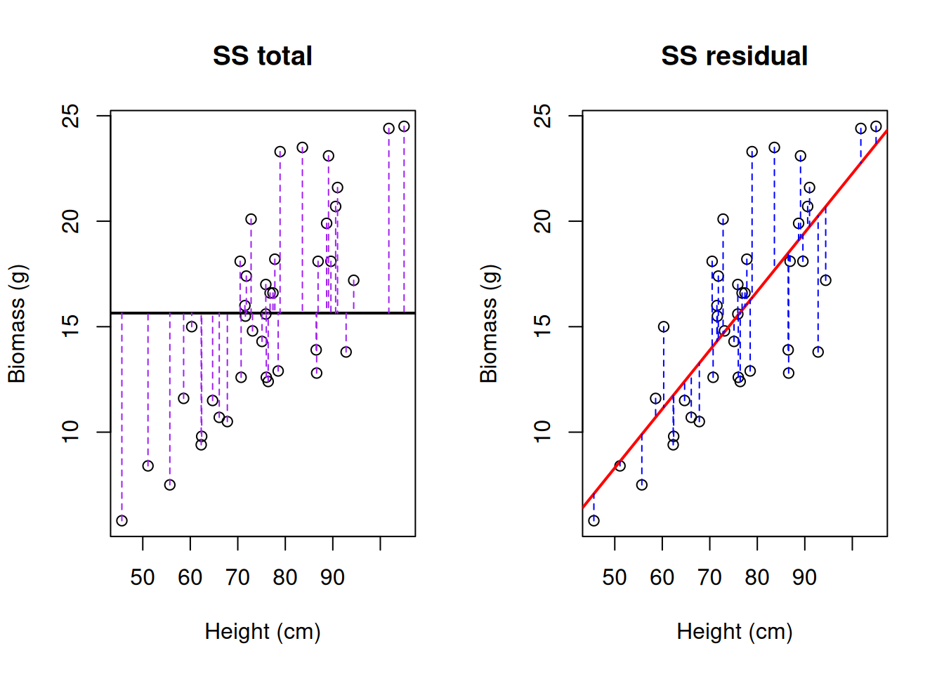
Demo: SS total vs SS residual, drawn
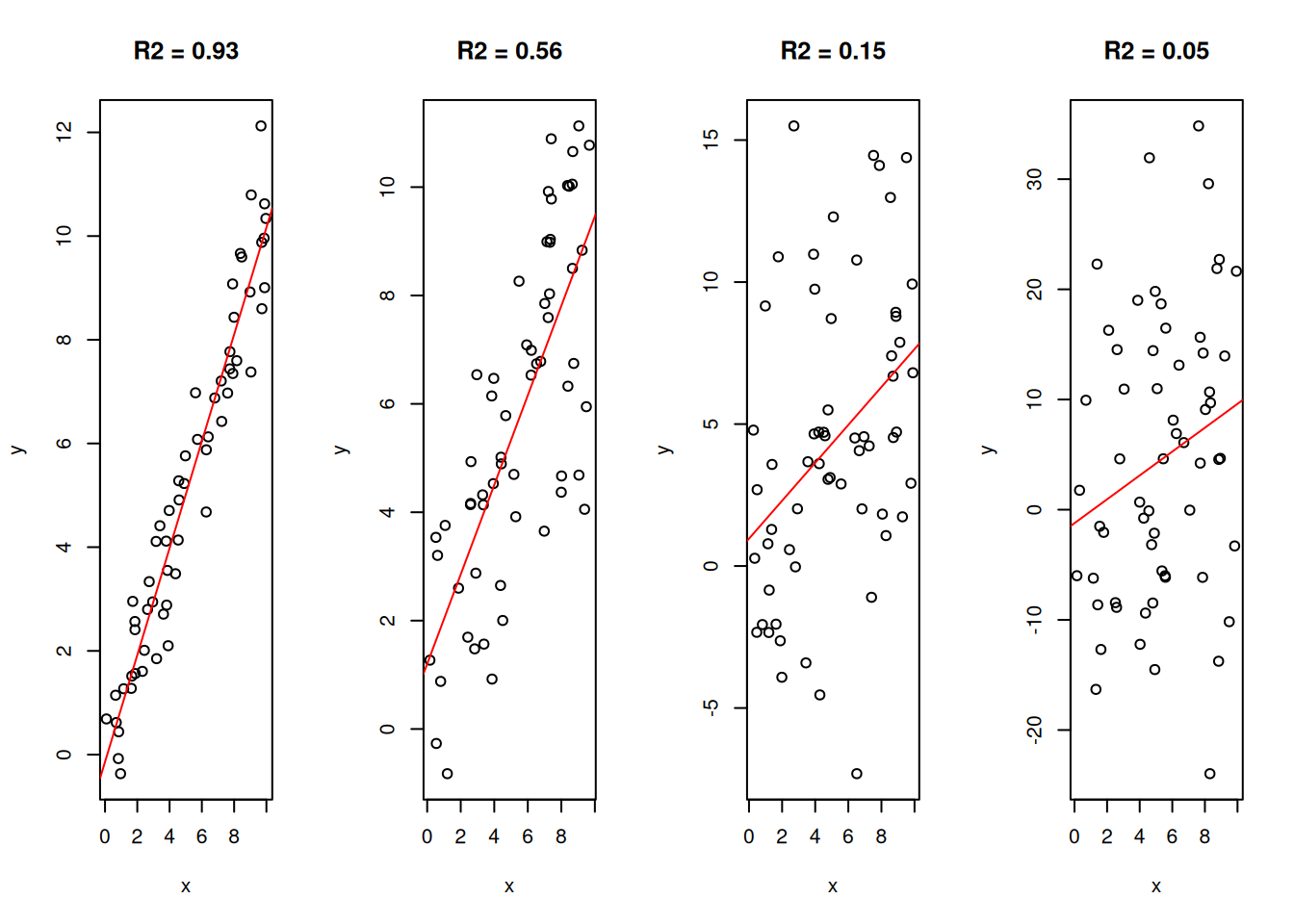
par(mfrow = c(1, 1))Demo: what different R2 values look like (simulated)
# what different R2 values look like (simulated: same slope, more or less noise)
set.seed(7)
par(mfrow = c(1, 4))
for (r2_target in c(0.9, 0.6, 0.3, 0.05)) {
  x <- runif(60, 0, 10)
  y <- x + rnorm(60, sd = sqrt((1 - r2_target) / r2_target * var(x)))
  plot(x, y, main = paste("R2 =", round(summary(lm(y ~ x))$r.squared, 2)))
  abline(lm(y ~ x), col = "red")
}
Demo: what different R2 values look like (simulated)
par(mfrow = c(1, 1))7) summary(): the full output
summary(model)
Call:
lm(formula = biomass ~ height, data = wheat)

Residuals:
    Min      1Q  Median      3Q     Max
-6.4505 -2.1590  0.0566  1.6519  6.9287

Coefficients:
            Estimate Std. Error t value Pr(>|t|)
(Intercept) -5.64783    2.89282  -1.952   0.0583 .
height       0.27908    0.03737   7.467 5.79e-09 ***
---
Signif. codes:  0 '***' 0.001 '**' 0.01 '*' 0.05 '.' 0.1 ' ' 1

Residual standard error: 3.083 on 38 degrees of freedom
Multiple R-squared:  0.5947,    Adjusted R-squared:  0.5841
F-statistic: 55.76 on 1 and 38 DF,  p-value: 5.785e-09
# the slope's t-test: estimate / SE, 38 df
coef(summary(model)) Estimate Std. Error t value Pr(>|t|)
(Intercept) -5.6478330 2.89282132 -1.952362 5.829150e-02
height 0.2790764 0.03737278 7.467371 5.785277e-09Demo: t and p by hand
0.27908 / 0.03737 # t[1] 7.468022Demo: t and p by hand
2 * pt(7.467, df = 38, lower.tail = FALSE) # two-sided p-value[1] 5.791889e-09# confidence interval for the slope: estimate +/- t * SE
confint(model) 2.5 % 97.5 %
(Intercept) -11.5040436 0.2083775
height 0.2034192 0.3547337Demo: the CI by hand, and where the SE comes from (a bootstrap)
0.27908 + c(-1, 1) * qt(0.975, df = 38) * 0.03737[1] 0.2034284 0.3547316Demo: the CI by hand, and where the SE comes from (a bootstrap)
# where the SE comes from: re-sample the plants and refit (a bootstrap)
set.seed(206)
slopes <- replicate(1000, {
  i <- sample(40, replace = TRUE)   # re-sample the plants
  coef(lm(biomass ~ height, data = wheat[i, ]))[2]
})
sd(slopes)        # spread of the slope
[1] 0.03301875Demo: the CI by hand, and where the SE comes from (a bootstrap)
summary(model)$coefficients[2, "Std. Error"][1] 0.03737278Demo: the CI by hand, and where the SE comes from (a bootstrap)
hist(slopes, xlab = "Slope (g per cm)", main = "1000 re-sampled slopes")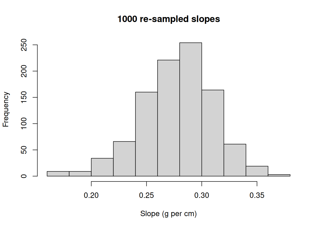
# the line with its confidence band
ggplot(wheat, aes(x = height, y = biomass)) +
  geom_point() +
  geom_smooth(method = "lm") +
  theme_classic()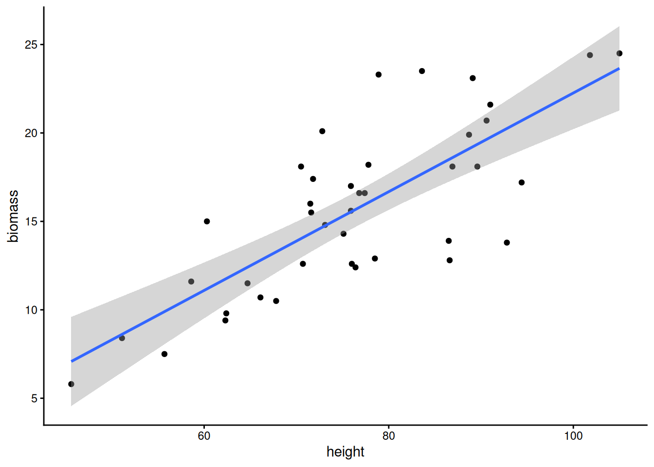
# two intervals: for the LINE (mean biomass at that height) and for ONE NEW PLANT
new <- data.frame(height = c(60, 80, 100))
predict(model, newdata = new, interval = "confidence")   # the line
fit lwr upr
1 11.09675 9.517423 12.67608
2 16.67828 15.652415 17.70415
3 22.25981 20.212925 24.30669predict(model, newdata = new, interval = "prediction") # a new plant: much wider fit lwr upr
1 11.09675 4.658465 17.53504
2 16.67828 10.352962 23.00360
3 22.25981 15.691172 28.82845# both bands on one plot: predict over a grid of heights, then draw the lines
grid <- data.frame(height = 45:110)
ci <- predict(model, grid, interval = "confidence")
pi <- predict(model, grid, interval = "prediction")
plot(wheat$height, wheat$biomass, xlab = "Height (cm)", ylab = "Biomass (g)", ylim = c(0, 36))
lines(grid$height, ci[, "fit"], col = "red", lwd = 2)
lines(grid$height, ci[, "lwr"], col = "red", lty = 2); lines(grid$height, ci[, "upr"], col = "red", lty = 2)
lines(grid$height, pi[, "lwr"], col = "blue", lty = 3); lines(grid$height, pi[, "upr"], col = "blue", lty = 3)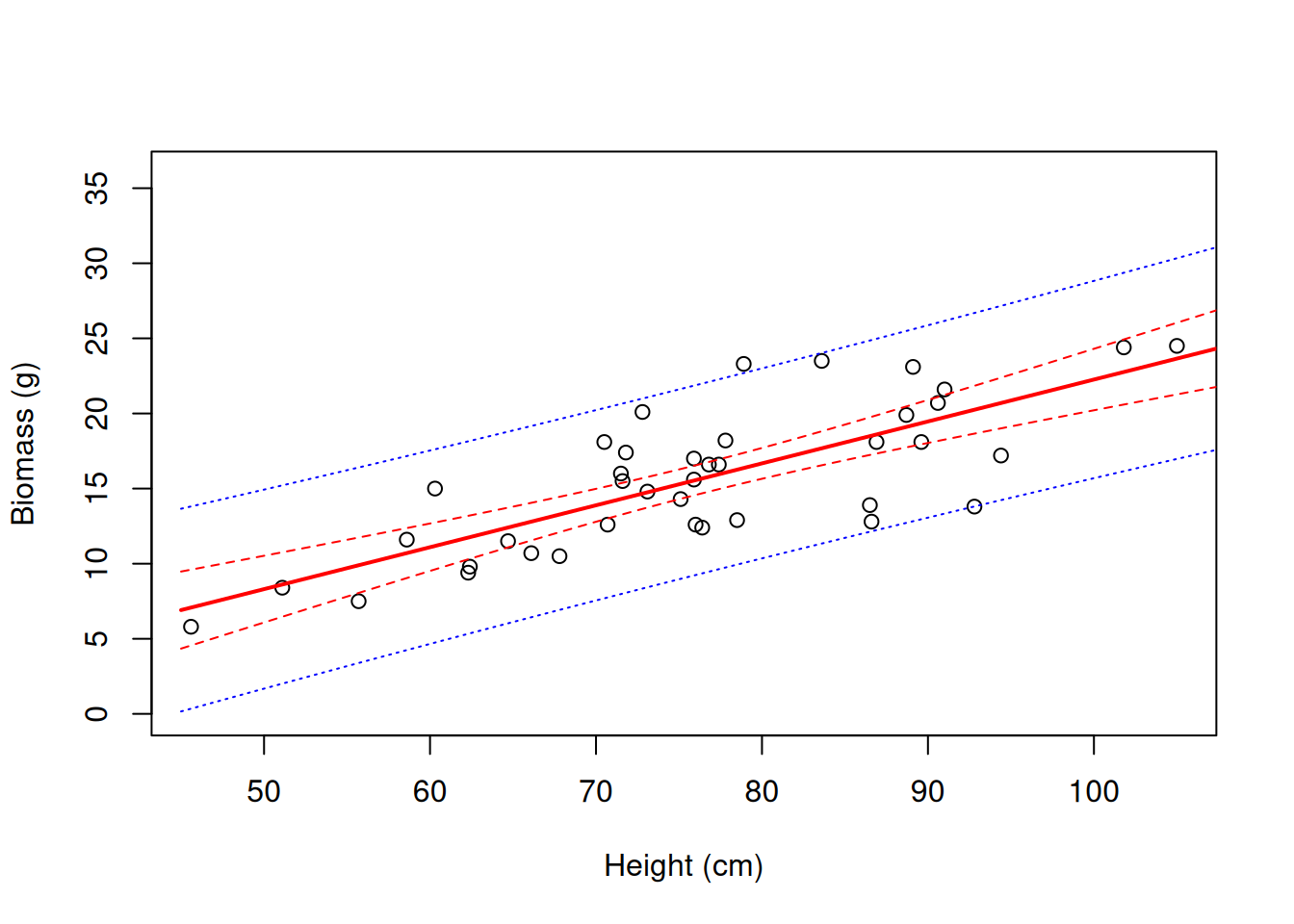
8) The F-test
Demo: F by hand from R2
r2 <- summary(model)$r.squared
k  <- 1            # predictors
n  <- nrow(wheat)  # plants
f  <- (r2 / k) / ((1 - r2) / (n - k - 1))
f
[1] 55.76163Demo: F by hand from R2
pf(f, k, n - k - 1, lower.tail = FALSE) # p-value[1] 5.785277e-09summary(model)$fstatistic value numdf dendf
55.76163 1.00000 38.00000 7.467^2 # one predictor: F = t^2[1] 55.75609Part C. Assumptions: what can go wrong
9) Diagnostic plots
par(mfrow = c(2, 2))   # four panels in one window
plot(model)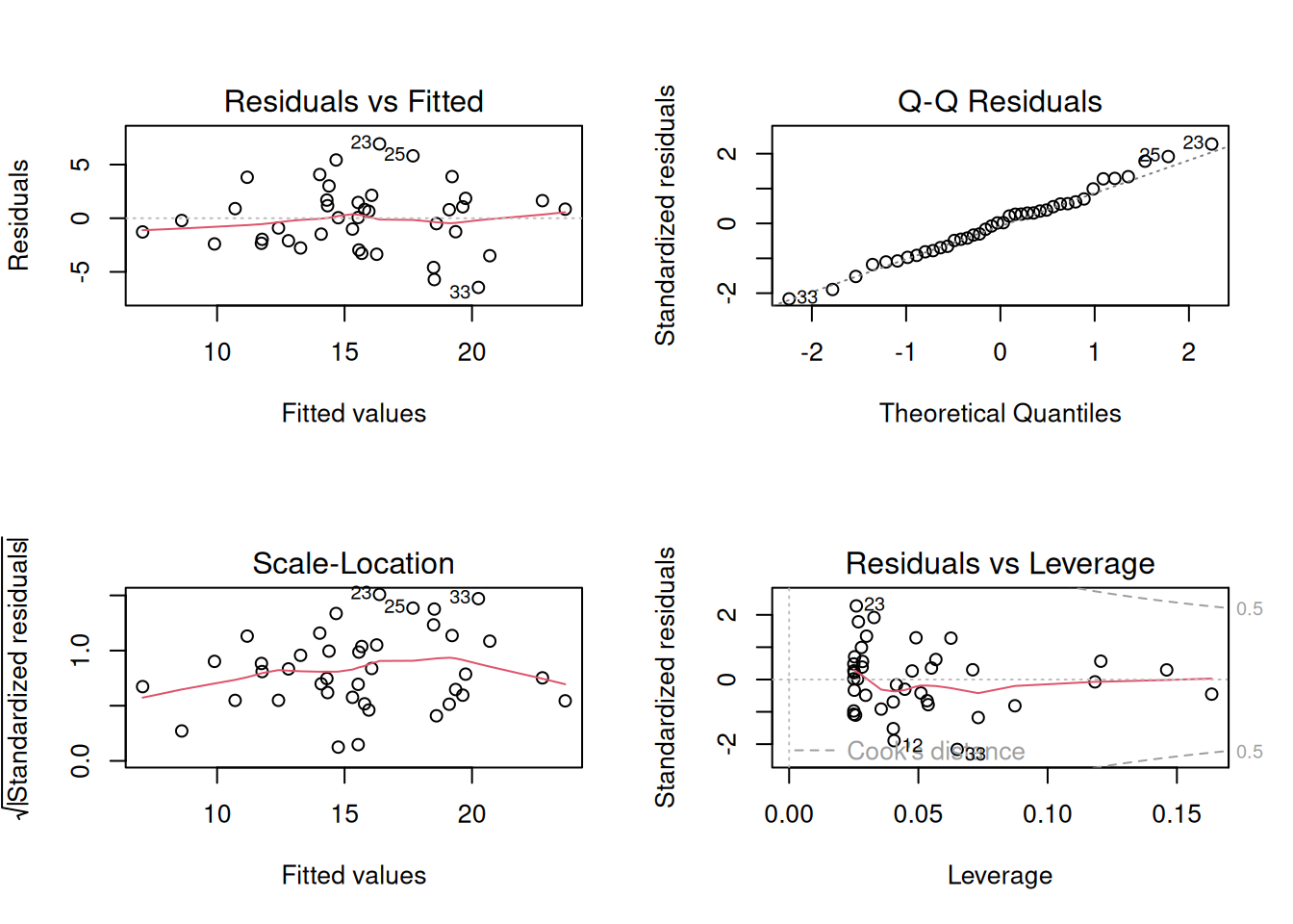
par(mfrow = c(1, 1))
# 1 residuals vs fitted: a shapeless cloud = linear
# 2 Q-Q: residuals on the line = normal
# 3 scale-location: flat = equal variance
# 4 residuals vs leverage: points with outsized pull on the line
Demo: the four residual-vs-fitted patterns to recognize (simulated)
# the four residual-vs-fitted patterns to recognize (simulated)
set.seed(11)
x <- runif(80, 0, 10)
par(mfrow = c(1, 4))
plot(x, rnorm(80), main = "fine", xlab = "fitted", ylab = "residual"); abline(h = 0, lty = 2)
plot(x, -((x - 5)^2) / 6 + 2 + rnorm(80, sd = 0.7), main = "curve", xlab = "fitted", ylab = "residual"); abline(h = 0, lty = 2)
plot(x, rnorm(80, sd = 0.2 + 0.3 * x), main = "fan", xlab = "fitted", ylab = "residual"); abline(h = 0, lty = 2)
plot(x, c(rnorm(79, sd = 0.8), 8), main = "outlier", xlab = "fitted", ylab = "residual"); abline(h = 0, lty = 2)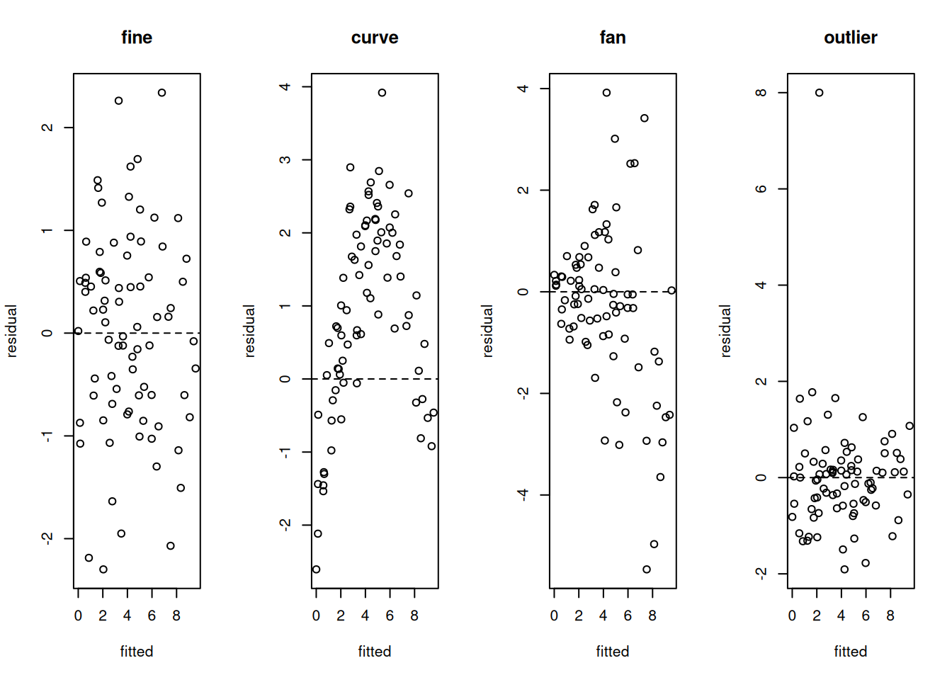
Demo: the four residual-vs-fitted patterns to recognize (simulated)
par(mfrow = c(1, 1))10) Violation 1: a curve
Demo: simulate growth that curves with water
set.seed(1)
water  <- runif(100, 0, 60)   # mm per week
growth <- 20 + 2.2 * water - 0.03 * water^2 +
  rnorm(100, sd = 4)
pots   <- data.frame(water, growth)
model_w <- lm(growth ~ water, data = pots)
summary(model_w)$r.squared[1] 0.38397plot(pots$water, pots$growth, xlab = "Water (mm/week)", ylab = "Growth (g)")
abline(model_w, col = "red", lwd = 2)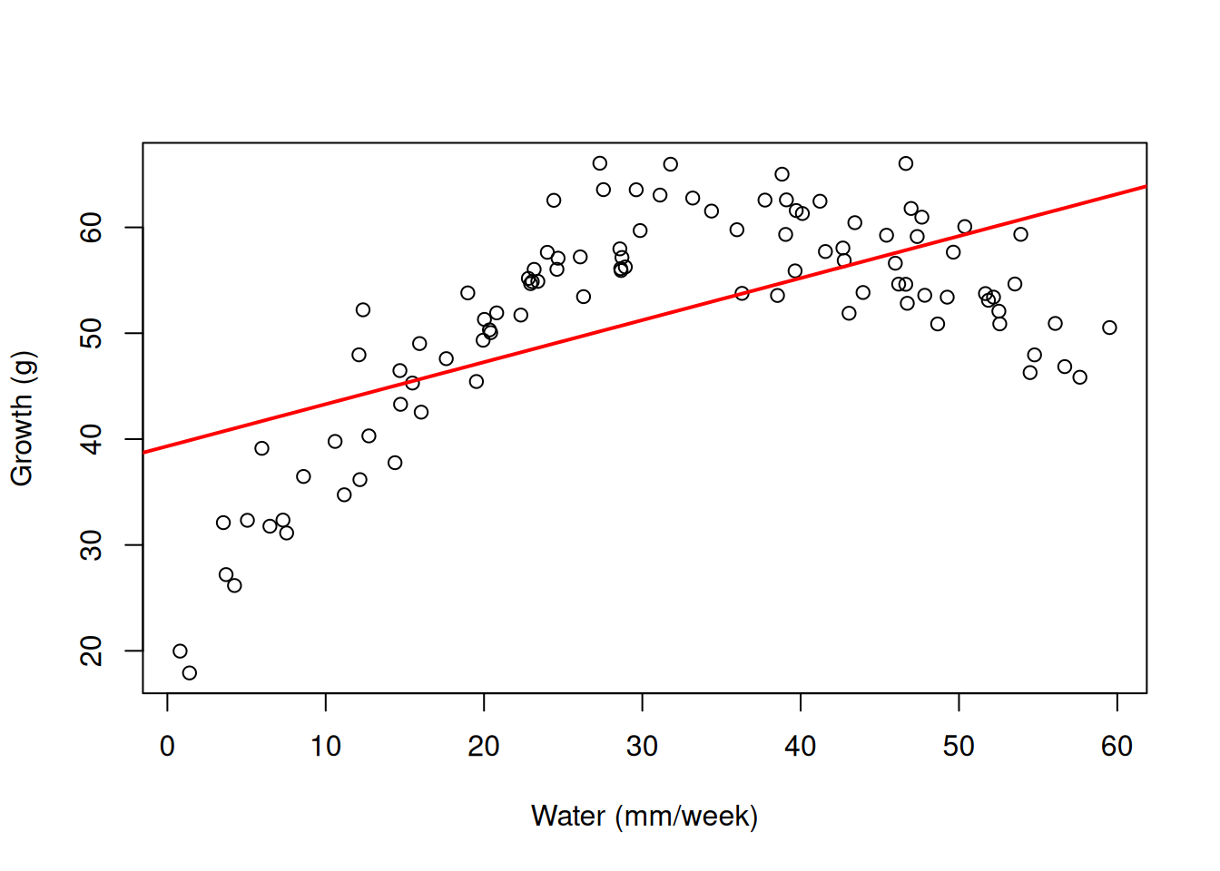
plot(model_w, which = 1) # residuals vs fitted: an arch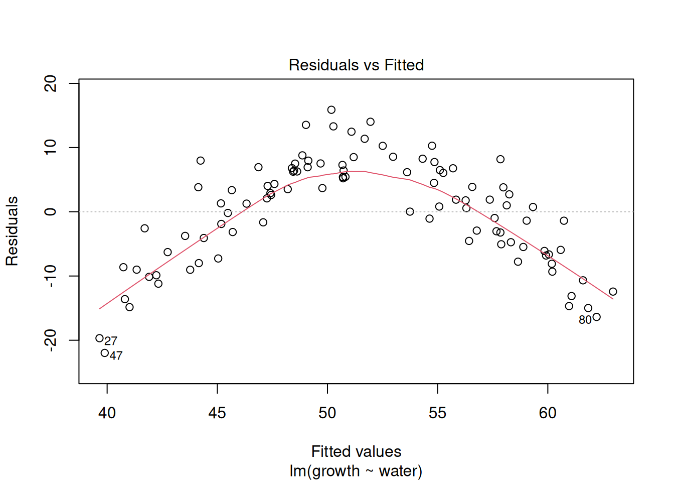
# fix: add a squared term (I() protects the ^ inside a formula)
model_w2 <- lm(growth ~ water + I(water^2), data = pots)
round(coef(model_w2), 3)
(Intercept) water I(water^2)
19.137 2.234 -0.030 summary(model_w2)$r.squared[1] 0.8674312# draw a curved fit: predict over a grid, then lines()
plot(pots$water, pots$growth, xlab = "Water (mm/week)", ylab = "Growth (g)")
lines(0:60, predict(model_w2, data.frame(water = 0:60)), col = "red", lwd = 2)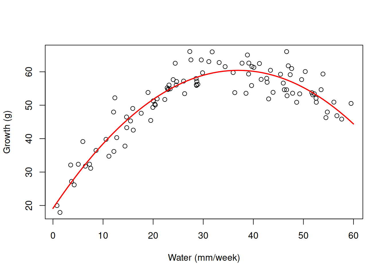
plot(model_w2, which = 1)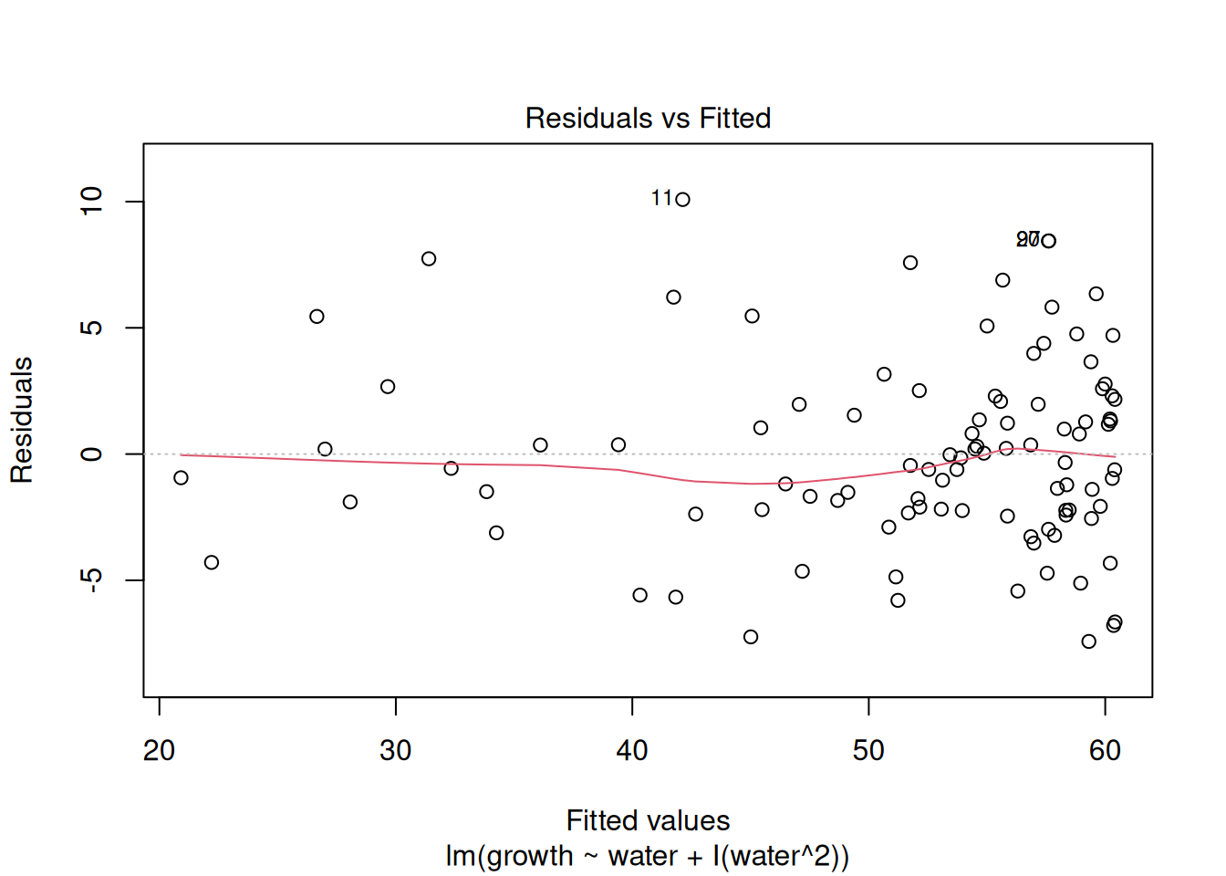
11) Violation 2: a fan
Demo: simulate yield whose spread grows with dose
set.seed(2)
dose  <- runif(150, 0, 60)   # fertilizer, kg/ha
yield <- exp(1.5 + 0.03 * dose + rnorm(150, sd = 0.25))
plots <- data.frame(dose, yield)
model_f <- lm(yield ~ dose, data = plots)
plot(plots$dose, plots$yield, xlab = "Fertilizer (kg/ha)", ylab = "Yield (t/ha)")
abline(model_f, col = "red", lwd = 2)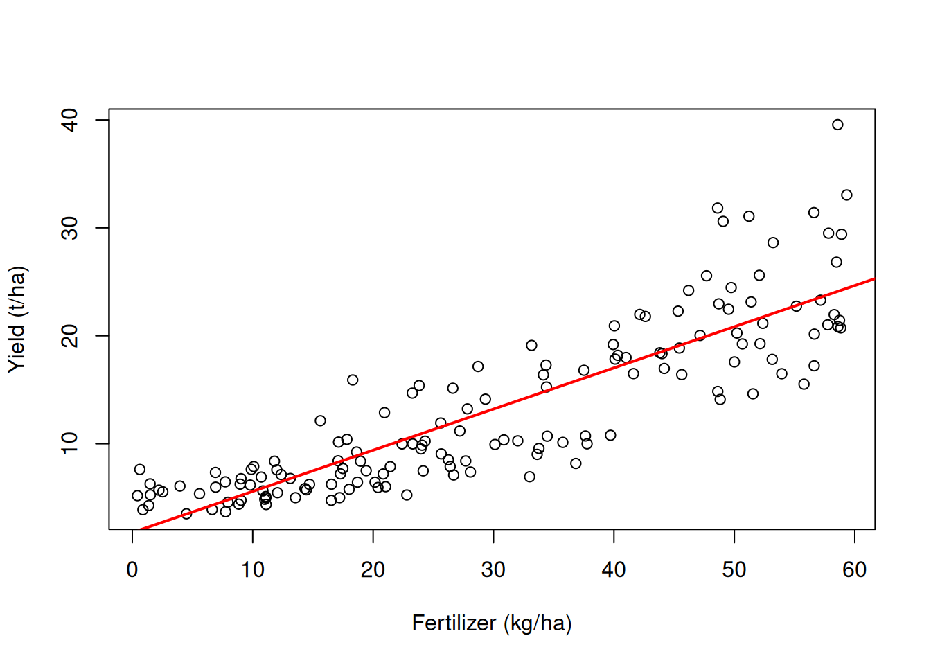
plot(model_f, which = 1) # the spread grows with the fitted value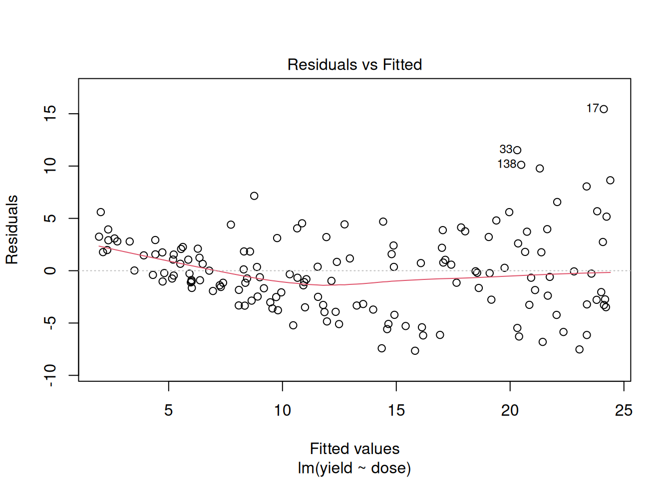
plot(model_f, which = 3) # scale-location: rising = unequal variance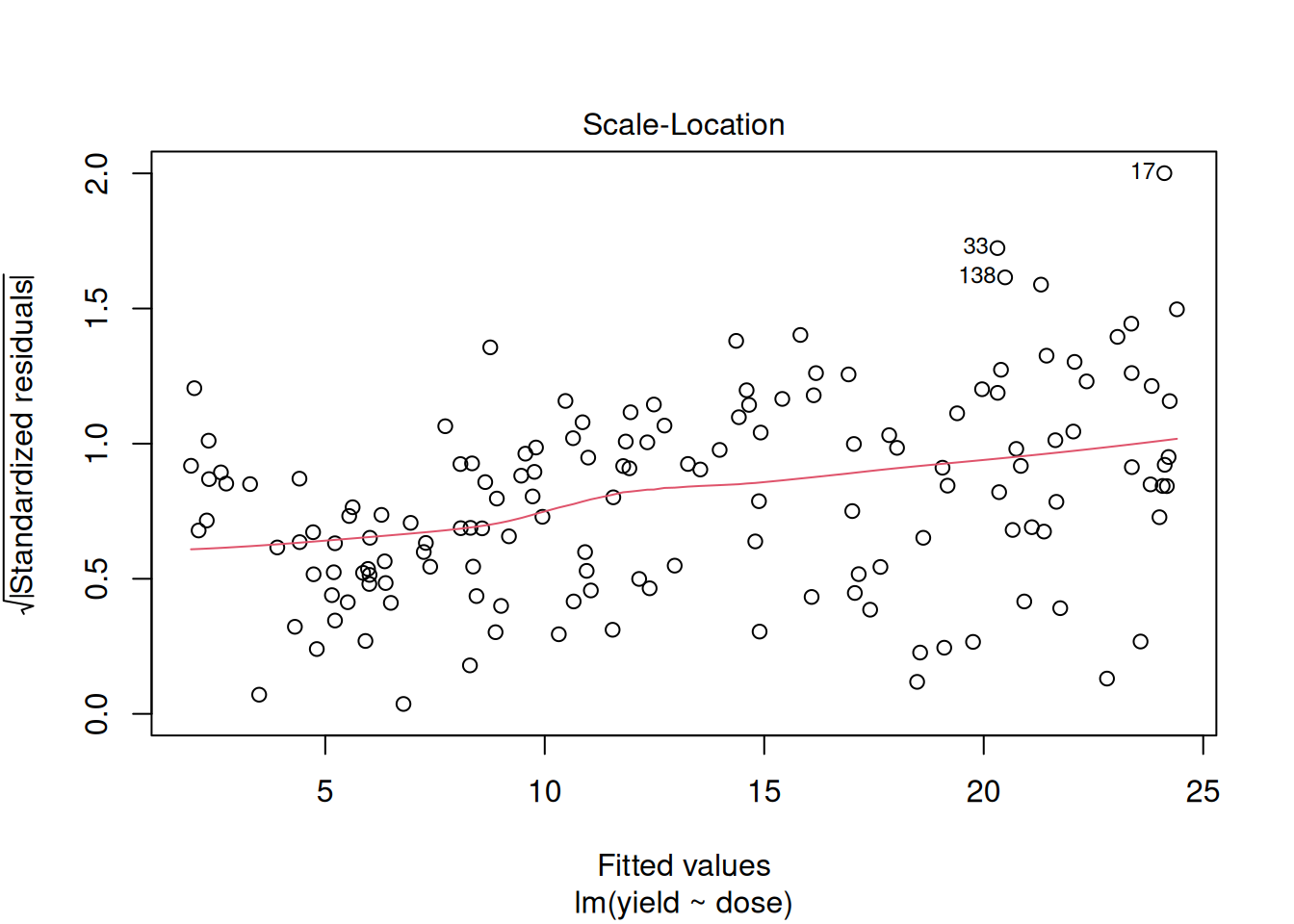
# fix: log the response. The slope becomes a percent change.
model_log <- lm(log(yield) ~ dose, data = plots)
round(coef(model_log), 3)
(Intercept) dose
1.50 0.03 exp(0.030) # x 1.03 per kg/ha: +3%[1] 1.030455plot(model_log, which = 1)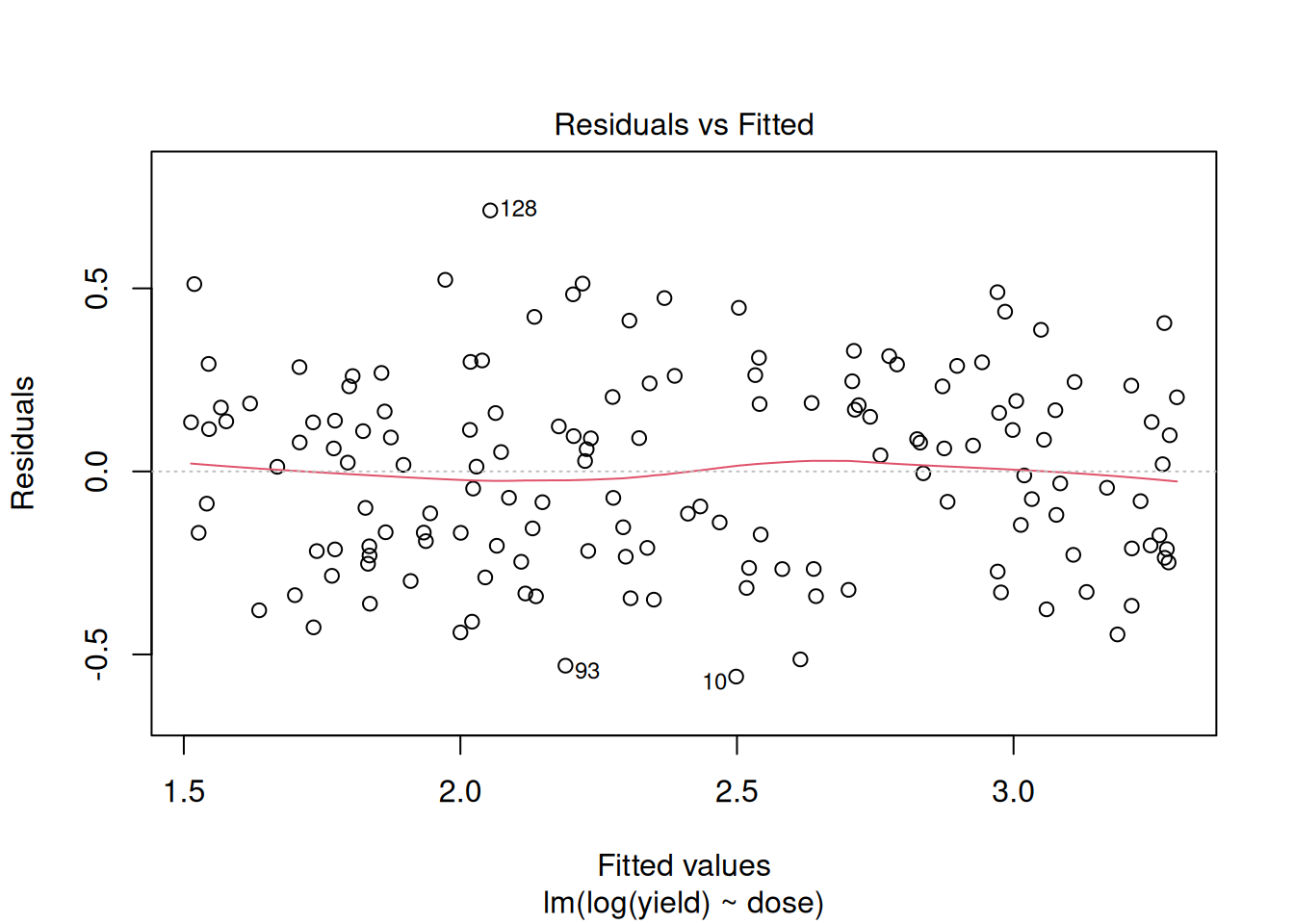
11b) Violation 3: residuals that are not normal (a count response)
Demo: simulate seed counts
set.seed(4)
size  <- runif(80, 1, 10)   # plant size
# seeds per plant: a count, many zeros
seeds <- rpois(80, lambda = exp(-1 + 0.35 * size))
pods  <- data.frame(size, seeds)
model_s <- lm(seeds ~ size, data = pods)
shapiro.test(resid(model_s))
    Shapiro-Wilk normality test

data:  resid(model_s)
W = 0.92704, p-value = 0.0002078par(mfrow = c(1, 2)); plot(model_s, which = 2); hist(resid(model_s)); par(mfrow = c(1, 1))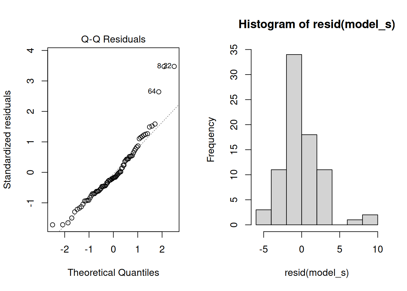
# the cure is a model for counts: a Poisson GLM (next week)
# glm(seeds ~ size, data = pods, family = poisson)
11c) Violation 4: one bad point (leverage, Cook’s distance)
Demo: plant a typo in the data
typo <- wheat
typo$biomass[7] <- 164   # 16.4 typed as 164
model_t <- lm(biomass ~ height, data = typo)
coef(model) # the real slope(Intercept) height
-5.6478330 0.2790764 coef(model_t) # with the typo(Intercept) height
6.0119191 0.1747512 plot(typo$height, typo$biomass); abline(model, col = "darkgreen", lwd = 2); abline(model_t, col = "red", lty = 2, lwd = 2)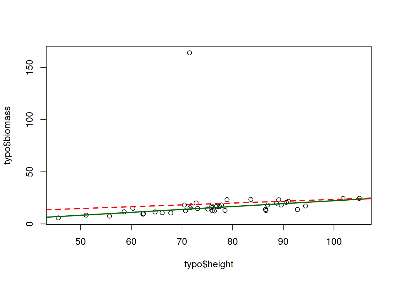
which.max(cooks.distance(model_t))7
7 max(cooks.distance(model_t))[1] 0.5460262plot(model_t, which = 5) # residuals vs leverage, with Cook's distance contours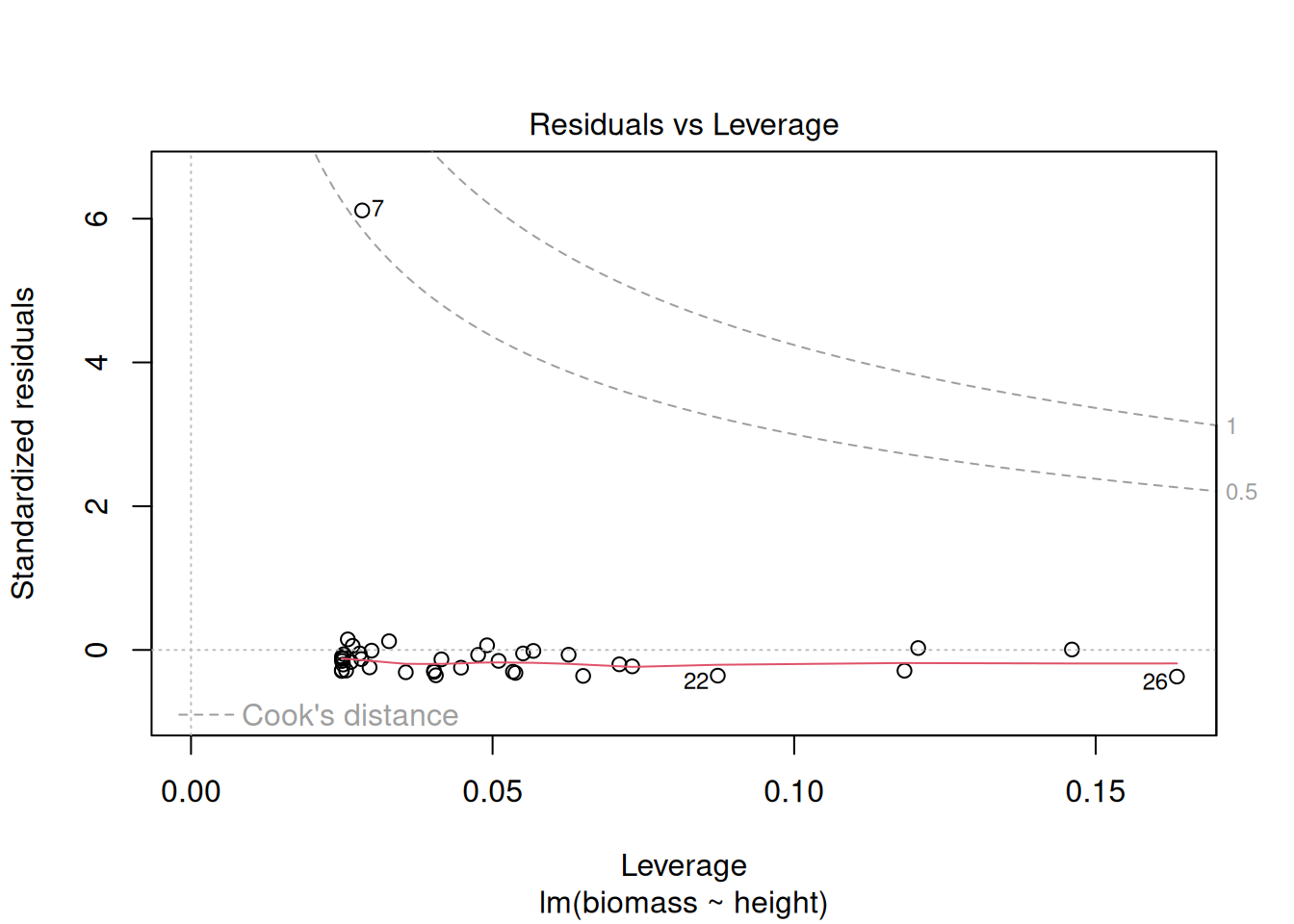
# the fix is not statistical: go back to the data sheet11d) Violation 5: not independent (pseudoreplication)
Demo: simulate 5 tillers in each of 8 pots
set.seed(22)
pot_h <- rnorm(8, sd = 4)     # each pot has its own soil...
pot_b <- rnorm(8, sd = 2.5)   # ...and its own luck
pot   <- rep(1:8, each = 5)   # 5 tillers per pot, 8 pots
height  <- 70 + pot_h[pot] + rnorm(40, sd = 3)
biomass <- 2 + 0.2 * height + pot_b[pot] + rnorm(40, 0, 1)
pots <- data.frame(pot, height, biomass)
# 40 tillers treated as 40 plants
model_p <- lm(biomass ~ height, data = pots)
round(coef(summary(model_p)), 3) Estimate Std. Error t value Pr(>|t|)
(Intercept) -0.757 3.925 -0.193 0.848
height 0.232 0.054 4.310 0.000# the honest version: one value per pot, n = 8
pot_means <- aggregate(cbind(height, biomass) ~ pot, pots, mean)
round(coef(summary(lm(biomass ~ height, pot_means))), 3) Estimate Std. Error t value Pr(>|t|)
(Intercept) -2.647 9.789 -0.27 0.796
height 0.259 0.135 1.92 0.103# the giveaway: residuals clump by pot
plot(fitted(model_p), resid(model_p), col = pots$pot, pch = 16); abline(h = 0, lty = 2)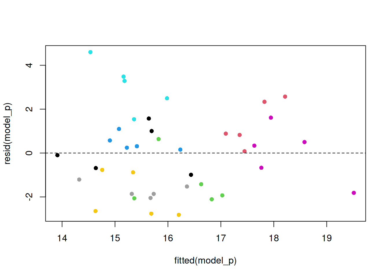
# (a mixed model with pot as a random effect is the Week 10 bonus)11e) Missing data: lm() drops rows silently
Demo: knock out three nitrogen values
wheat_na <- wheat
# three plants were not measured
wheat_na$nitrogen[c(3, 11, 25)] <- NAcolSums(is.na(wheat_na)) plant water nitrogen height biomass predicted residual
0 0 3 0 0 0 0 model_na <- lm(biomass ~ height + nitrogen, data = wheat_na)
nobs(model_na) # rows actually used[1] 37length(resid(model_na)) # shorter than the data frame![1] 37sum(complete.cases(wheat_na))[1] 37model_na <- lm(biomass ~ height + nitrogen, wheat_na,
na.action = na.exclude)
# padded with NA: lines up with the data
length(resid(model_na))[1] 40wheat_na$residual <- resid(model_na)Part D. Multiple regression
12) Two predictors
model2 <- lm(biomass ~ height + nitrogen, data = wheat)
summary(model2)
Call:
lm(formula = biomass ~ height + nitrogen, data = wheat)

Residuals:
    Min      1Q  Median      3Q     Max
-5.2589 -1.3734 -0.1355  1.2666  4.4950

Coefficients:
            Estimate Std. Error t value Pr(>|t|)
(Intercept) -2.72580    2.45074  -1.112    0.273
height       0.19902    0.03538   5.625 2.02e-06 ***
nitrogen     0.04862    0.01087   4.472 7.11e-05 ***
---
Signif. codes:  0 '***' 0.001 '**' 0.01 '*' 0.05 '.' 0.1 ' ' 1

Residual standard error: 2.517 on 37 degrees of freedom
Multiple R-squared:  0.7369,    Adjusted R-squared:  0.7227
F-statistic: 51.82 on 2 and 37 DF,  p-value: 1.87e-11
# each slope: the effect of that predictor holding the other fixed# the fitted plane (needs scatterplot3d)
library(scatterplot3d)
s3 <- scatterplot3d(wheat$height, wheat$nitrogen, wheat$biomass, pch = 16,
xlab = "Height (cm)", ylab = "Nitrogen (kg/ha)", zlab = "Biomass (g)")
s3$plane3d(model2)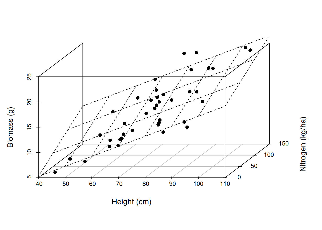
# "holding the other fixed": the height slope at three nitrogen levels
grid <- expand.grid(height = c(50, 100), nitrogen = c(25, 75, 125))
grid$biomass <- predict(model2, grid)
grid
height nitrogen biomass
1 50 25 8.440803
2 100 25 18.391817
3 50 75 10.871970
4 100 75 20.822985
5 50 125 13.303137
6 100 125 23.254152Demo: parallel lines, one per nitrogen level
# the same slope for height at each nitrogen level: parallel lines
plot(wheat$height, wheat$biomass, xlab = "Height (cm)", ylab = "Biomass (g)",
     col = c("salmon", "darkgreen", "steelblue")[cut(wheat$nitrogen, c(-1, 50, 100, 151))], pch = 16)
for (nit in c(25, 75, 125)) {
  abline(coef(model2)[1] + coef(model2)[3] * nit, coef(model2)[2],
         col = c("salmon", "darkgreen", "steelblue")[match(nit, c(25, 75, 125))], lwd = 2)
}
legend("topleft", legend = c("low N", "mid N", "high N"), col = c("salmon", "darkgreen", "steelblue"), lwd = 2, bty = "n")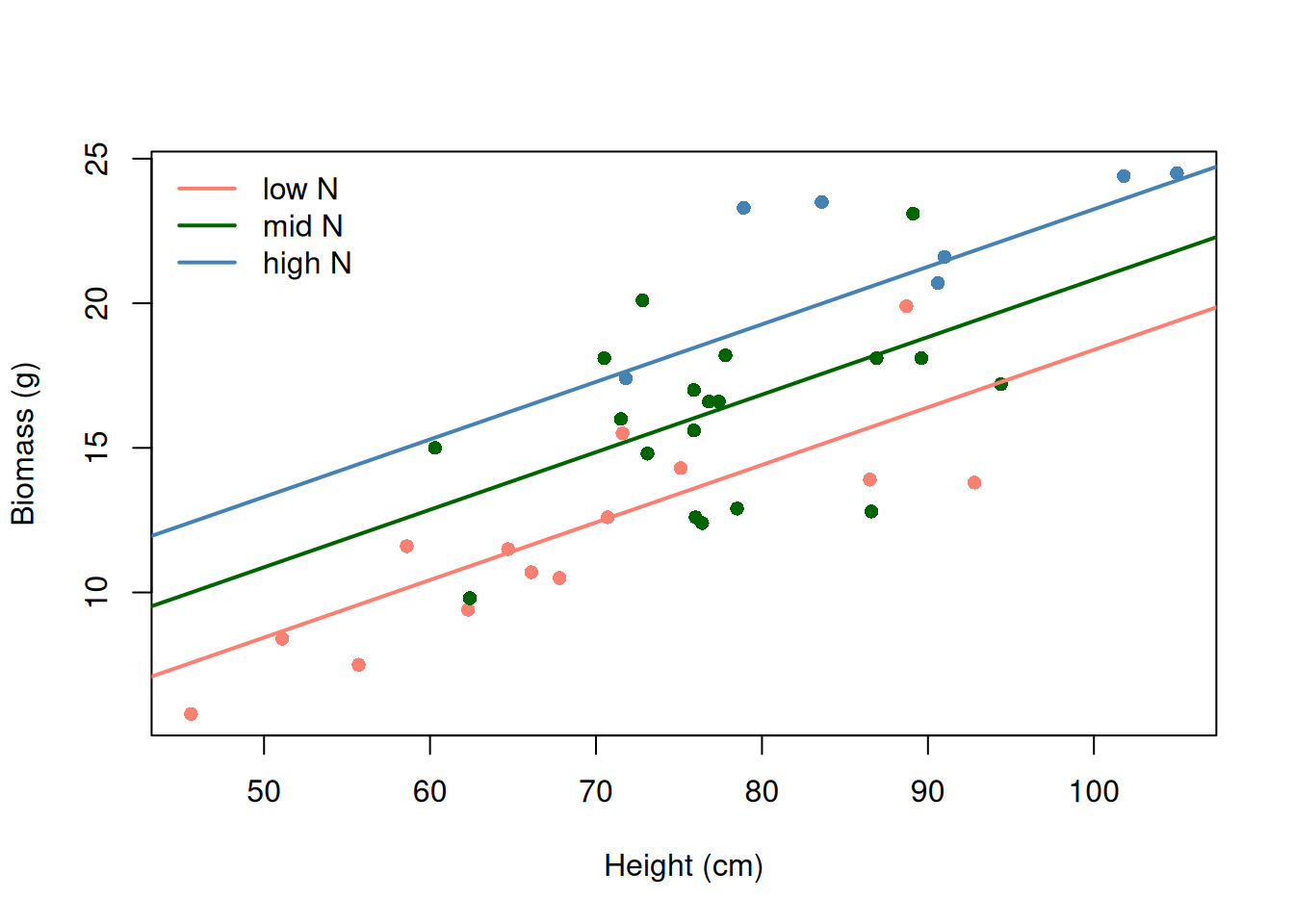
# why the height slope changed
coef(model)    # biomass ~ height
(Intercept) height
-5.6478330 0.2790764 coef(model2) # biomass ~ height + nitrogen(Intercept) height nitrogen
-2.72579601 0.19902030 0.04862335 cor(wheat$height, wheat$nitrogen)[1] 0.506009213) R2 only goes up: adjusted R2
Demo: add a predictor that is pure noise
set.seed(206)
wheat$noise <- rnorm(40)   # a predictor that is pure noise
r2 <- function(m) summary(m)$r.squared
r2(lm(biomass ~ height, wheat))
[1] 0.594717Demo: add a predictor that is pure noise
r2(lm(biomass ~ height + nitrogen, wheat))[1] 0.7369115Demo: add a predictor that is pure noise
r2(lm(biomass ~ height + nitrogen + noise, wheat))[1] 0.7489497Demo: add a predictor that is pure noise
adj <- function(m) summary(m)$adj.r.squared
adj(lm(biomass ~ height + nitrogen + noise, wheat))
[1] 0.728028913b) Does nitrogen earn its place? Nested models
anova(model, model2) # does nitrogen improve the fit?Analysis of Variance Table
Model 1: biomass ~ height
Model 2: biomass ~ height + nitrogen
Res.Df RSS Df Sum of Sq F Pr(>F)
1 38 361.23
2 37 234.49 1 126.74 19.998 7.112e-05 ***
---
Signif. codes: 0 '***' 0.001 '**' 0.01 '*' 0.05 '.' 0.1 ' ' 1Demo: F = t^2 when one term is added
coef(summary(model2))["nitrogen", "t value"]^2 # = F (one term added)[1] 19.99782# the F-test earns its keep when several terms are added at once:
# a 3-level factor, x + I(x^2), a block of variables
anova(model2) # sequential: height, then nitrogenAnalysis of Variance Table
Response: biomass
Df Sum Sq Mean Sq F value Pr(>F)
height 1 530.07 530.07 83.639 4.941e-11 ***
nitrogen 1 126.74 126.74 19.998 7.112e-05 ***
Residuals 37 234.49 6.34
---
Signif. codes: 0 '***' 0.001 '**' 0.01 '*' 0.05 '.' 0.1 ' ' 1# the other order
anova(lm(biomass ~ nitrogen + height, wheat))Analysis of Variance Table
Response: biomass
Df Sum Sq Mean Sq F value Pr(>F)
nitrogen 1 456.26 456.26 71.992 3.306e-10 ***
height 1 200.55 200.55 31.645 2.020e-06 ***
Residuals 37 234.49 6.34
---
Signif. codes: 0 '***' 0.001 '**' 0.01 '*' 0.05 '.' 0.1 ' ' 1# each term given the others (= the t-tests)
drop1(model2, test = "F")Single term deletions
Model:
biomass ~ height + nitrogen
Df Sum of Sq RSS AIC F value Pr(>F)
<none> 234.49 76.741
height 1 200.55 435.04 99.463 31.645 2.020e-06 ***
nitrogen 1 126.74 361.23 92.025 19.998 7.112e-05 ***
---
Signif. codes: 0 '***' 0.001 '**' 0.01 '*' 0.05 '.' 0.1 ' ' 114) The F-test with k = 2
Demo: F by hand with two predictors
r2 <- summary(model2)$r.squared
k <- 2; n <- 40
f <- (r2 / k) / ((1 - r2) / (n - k - 1))
f
[1] 51.81853Demo: F by hand with two predictors
pf(f, k, n - k - 1, lower.tail = FALSE)[1] 1.870191e-1115) Interactions
# y ~ x1 * x2  is  x1 + x2 + x1:x2
model_int <- lm(biomass ~ height * nitrogen, data = wheat)
round(coef(summary(model_int)), 4)
Estimate Std. Error t value Pr(>|t|)
(Intercept) -2.9686 3.8008 -0.7810 0.4399
height 0.2022 0.0523 3.8688 0.0004
nitrogen 0.0532 0.0549 0.9679 0.3395
height:nitrogen -0.0001 0.0007 -0.0844 0.9332# height:nitrogen p = 0.93: no interaction here; keep the simpler modelDemo: what an interaction looks like (simulated)
# what an interaction looks like (simulated): the slope of x1 depends on x2
set.seed(5)
x1 <- runif(60, 0, 10); x2 <- rep(c("low", "high"), each = 30)
y_no  <- 2 + 1 * x1 + ifelse(x2 == "high", 3, 0) + rnorm(60)             # parallel
y_int <- 2 + ifelse(x2 == "high", 2, 0.4) * x1 + rnorm(60)               # not parallel
par(mfrow = c(1, 2))
plot(x1, y_no, col = ifelse(x2 == "high", "darkcyan", "salmon"), pch = 16, main = "no interaction")
plot(x1, y_int, col = ifelse(x2 == "high", "darkcyan", "salmon"), pch = 16, main = "interaction")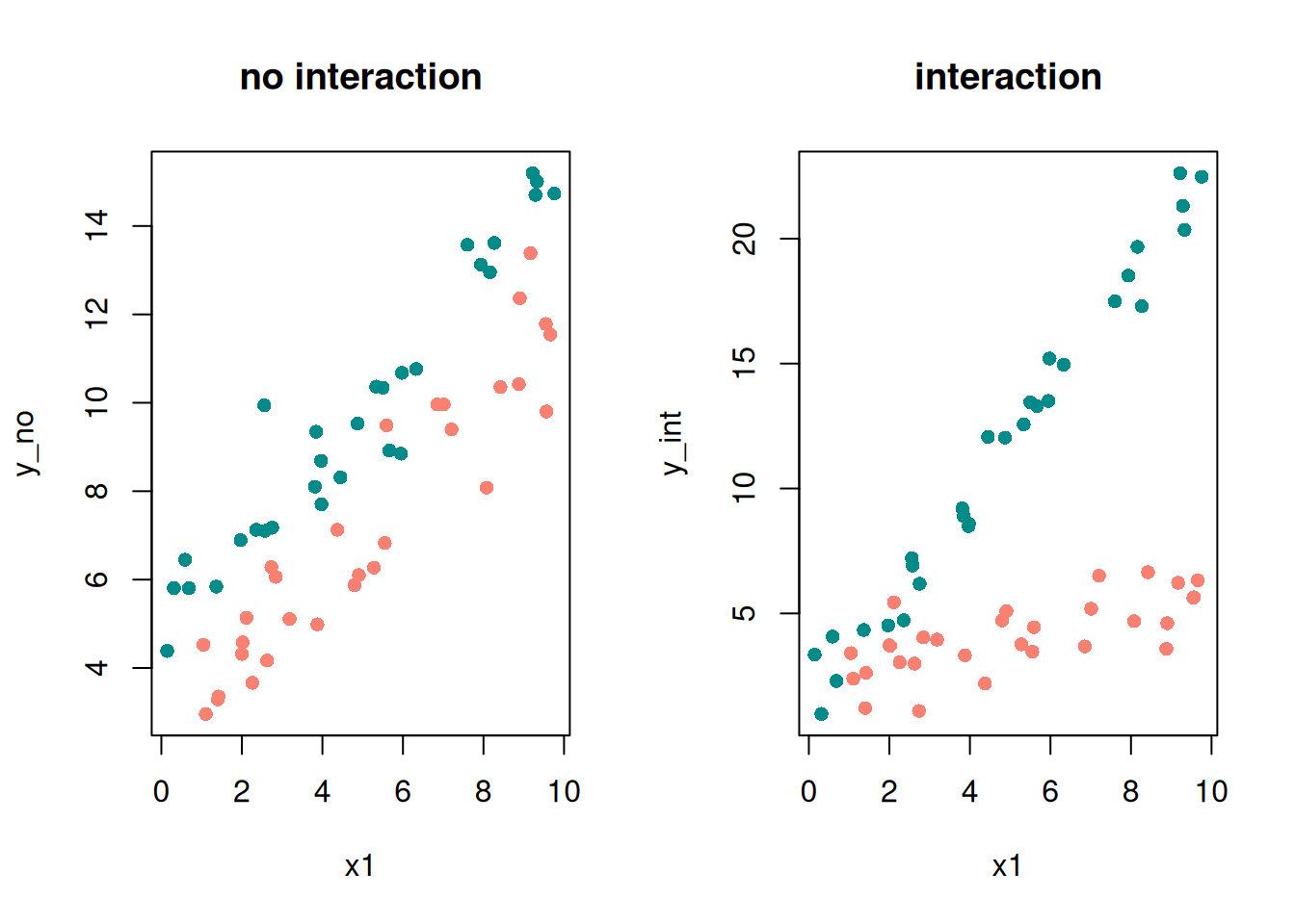
Demo: what an interaction looks like (simulated)
par(mfrow = c(1, 1))
round(coef(summary(lm(y_int ~ x1 * x2))), 3)   # the x1:x2 term is the interaction
Estimate Std. Error t value Pr(>|t|)
(Intercept) 1.142 0.358 3.193 0.002
x1 2.161 0.064 33.958 0.000
x2low 1.214 0.515 2.358 0.022
x1:x2low -1.815 0.090 -20.244 0.000A real one: a fertilizer x irrigation trial.
Demo: simulate the fertilizer x irrigation trial
set.seed(18)
trial <- data.frame(nitrogen = runif(60, 0, 150),
                    water    = runif(60, 10, 50))
trial$yield <- 5 + 0.01 * trial$nitrogen + 0.05 * trial$water +
  0.002 * trial$nitrogen * trial$water + rnorm(60, sd = 1.2)
model_nw <- lm(yield ~ nitrogen * water, data = trial)
round(coef(summary(model_nw)), 4) Estimate Std. Error t value Pr(>|t|)
(Intercept) 5.2123 0.6944 7.5061 0.0000
nitrogen 0.0068 0.0091 0.7506 0.4560
water 0.0403 0.0211 1.9144 0.0607
nitrogen:water 0.0021 0.0003 7.5646 0.0000# the nitrogen slope at three water levels: b1 + b3 * water
coef(model_nw)["nitrogen"] + coef(model_nw)["nitrogen:water"] * c(15, 30, 45)[1] 0.03849851 0.07019931 0.10190010# always plot an interaction: predict over a grid, one line per water level
g <- expand.grid(nitrogen = c(0, 150), water = c(15, 30, 45))
g$yield <- predict(model_nw, g)
plot(trial$nitrogen, trial$yield, xlab = "Nitrogen (kg/ha)", ylab = "Yield (t/ha)")
for (w in c(15, 30, 45)) lines(g$nitrogen[g$water == w], g$yield[g$water == w], lwd = 2, col = c("salmon", "darkgreen", "steelblue")[match(w, c(15, 30, 45))])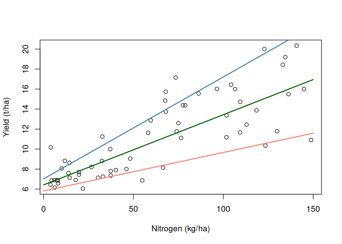
# centring: the product term overlaps its parts
library(car)    # vif()
vif(model_nw)
nitrogen water nitrogen:water
8.978014 2.850287 10.761527 trial$nitrogen_c <- trial$nitrogen - mean(trial$nitrogen)
trial$water_c <- trial$water - mean(trial$water)
model_nwc <- lm(yield ~ nitrogen_c * water_c, data = trial)
vif(model_nwc) # centred: the overlap is gone nitrogen_c water_c nitrogen_c:water_c
1.013733 1.001760 1.015259 # same interaction; main effects now at the mean
round(coef(model_nwc), 4) (Intercept) nitrogen_c water_c nitrogen_c:water_c
11.1270 0.0741 0.1725 0.0021 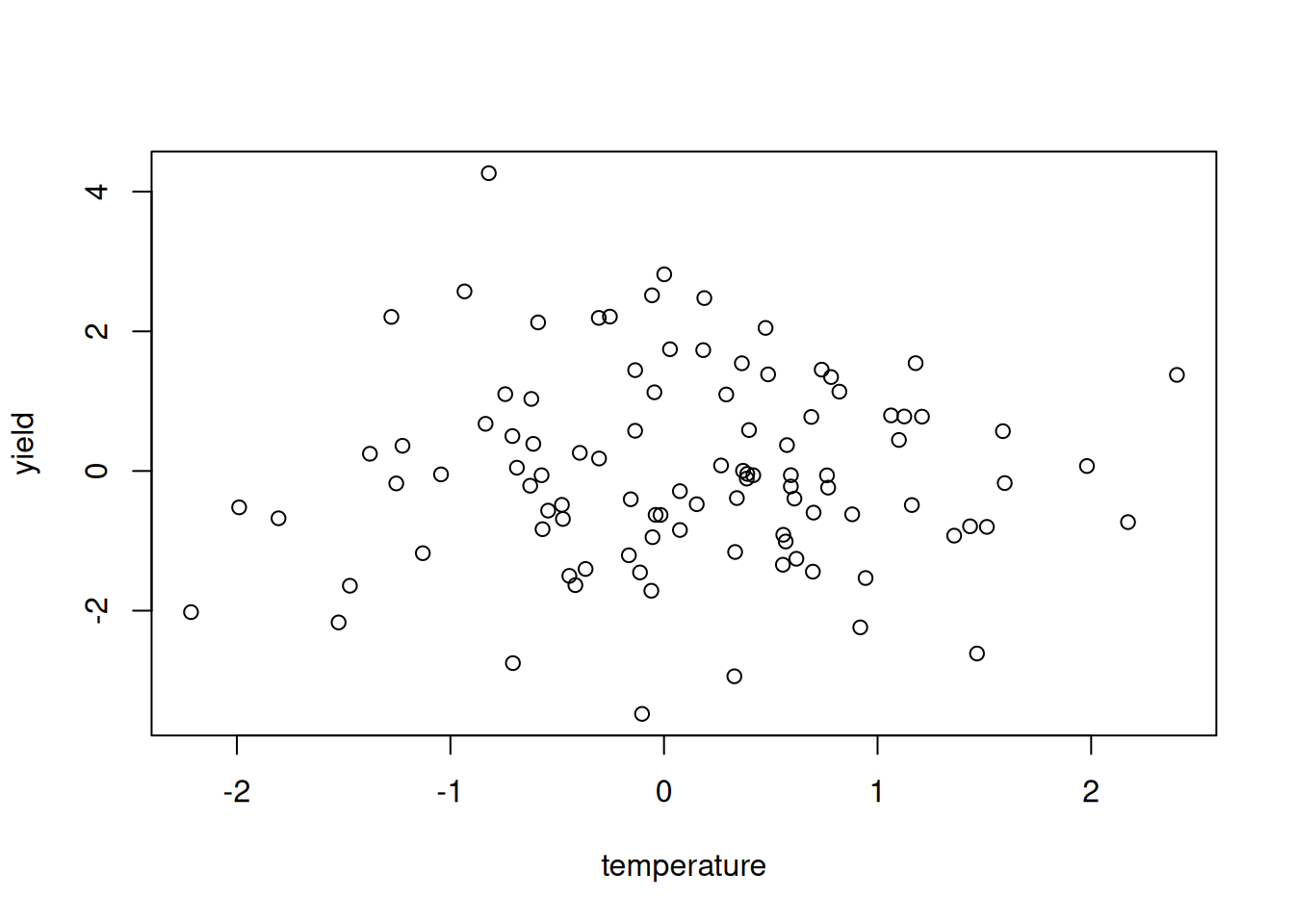
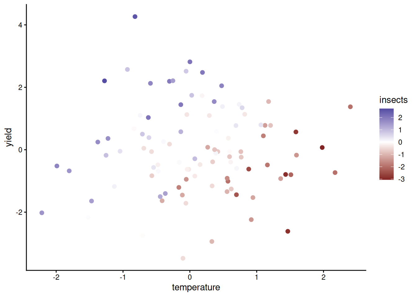
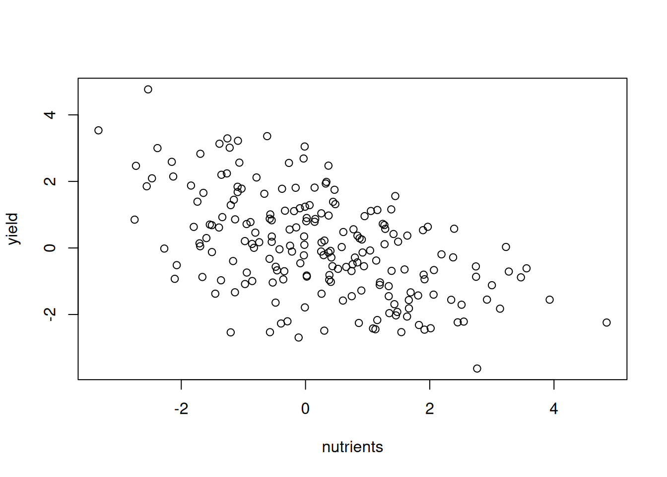
Part F. Under the hood, and reporting
20) The design matrix
Demo: least squares in one line of matrix algebra
head(model.matrix(model2), 4) # a column of 1s for the intercept (Intercept) height nitrogen
1 1 86.9 89
2 1 71.6 6
3 1 73.1 66
4 1 75.9 70Demo: least squares in one line of matrix algebra
# least squares in one line of matrix algebra: (X'X)^-1 X'y
X <- model.matrix(model2); y <- wheat$biomass
solve(t(X) %*% X) %*% t(X) %*% y
[,1]
(Intercept) -2.72579601
height 0.19902030
nitrogen 0.04862335Demo: least squares in one line of matrix algebra
coef(model2)(Intercept) height nitrogen
-2.72579601 0.19902030 0.04862335 21) Reporting: effect size in units, CI, R2, n
coef(model)[2]; confint(model)[2, ]; summary(model)$r.squared; nrow(wheat) height
0.2790764 2.5 % 97.5 %
0.2034192 0.3547337 [1] 0.594717[1] 40# "Biomass increased with height (0.28 g per cm, 95% CI 0.20 to 0.35;
# t38 = 7.5, p < 0.001). Height explained 59% of the variation in
# biomass (R2 = 0.59, n = 40)."# which predictor matters more? standardize both: slopes in SD units
model_std <- lm(scale(biomass) ~ scale(height) +
scale(nitrogen), data = wheat)
round(coef(model_std), 2) # slopes in SD units (Intercept) scale(height) scale(nitrogen)
0.00 0.55 0.44